GaWC Research Bulletin 196

This Research Bulletin has been published in Urban Geography, 28 (3), (2007), 232-248.

Please refer to the published version when quoting the paper.

(Z)

Comparing Airline Passenger Destinations with Global Service Connectivities: A Worldwide Empirical Study of 214 Cities¹

P.J. Taylor^*, B. Derudder^** and F. Witlox^***

Abstract

This research note compares two commonly employed data sources in world city research, i.e. (i) data on corporate organization and (ii) information on air passenger flows. For both types of data we construct connectivity measures, which are then compared through a standard least squares regression analysis. The empirical specifics that emerge from our analysis are discussed through an examination of the regression residuals, which we interpret in terms of cities being under-served and/or over-visited or being over-serviced and/or under-visited. Our findings are generalised by discussing them against the backdrop of Castells’ description of contemporary globalization as a ‘network society’.

INTRODUCTION

This research note aims to contribute to the literature that attempts to measure the dynamics of globalization, of which the rise of a ‘world city network’ has been one the key identifiers. Through the 1990s one particular criticism of this world city literature became commonplace: there was a severe empirical deficit as regards inter-city relations (e.g. Knox, 1995; Smith and Timberlake, 1995a, 1995b; Taylor, 1997, 1999, 2000; Beaverstock et al., 2000a, 2000b). That this could be fundamentally debilitating was abundantly clear because the raison d’être of these cities is their worldwide interconnections. But this potential evidential crisis has been averted in recent years. Two separate and distinctive solutions to the problem have been developed (Derudder, 2006): analysing worldwide corporate organisation (e.g. Godfrey and Zhou, 1999), and describing the infrastructure that has enabled that organisation to go global (e.g. Graham, 1999). It is the purpose of this research note to compare these two solutions by focusing on the most frequent manifestations of each approach, namely the organization of advanced producer service firms and the distribution of commercial airline traffic. We use a basic quantitative evaluation of the relation between results of these two approaches and explore some of the empirical specifics that emerge from this analysis.

The use of standard air travel statistics as the common ‘data of choice’ for researching worldwide inter-city relations has been largely a data-led decision since information on international flows is publicly available (Keeling, 1995). In addition, however, these data with their description of flows between city airports have been popular because they provide concrete manifestations of inter-city flows that are relatively easy to analyse and interpret. The main problem with these standard data sources is that they detail international rather than global flows (thus ‘downgrading’ New York with its numerous domestic flights) and that they take the hub function of airports into account (thus ‘upgrading’ London with its numerous (non-domestic) onward connection flights). We overcome these problems by using a unique set of global passenger origin and destination data introduced in Derudder and Witlox (2005). The reason for the popularity of using advanced producer service firms in the corporate organisation approach has been a more theoretical choice, deriving from Sassen’s (1991, 2001) identification of the ‘global city’. Here she explicitly identifies leading financial and business service firms as critical to global city formation. Using this argument GaWC research has analysed the office networks of such firms across cities to describe a ‘world city network’ (Taylor et al., 2003; Taylor 2004). It is the results from the latter that are compared to the air passenger data below.

Sassen’s work has also been used by Castells (1996, 2001) as a prime global illustration of his concept of a social spatial construction he calls the ‘space of flows’. This is central to his conceptualization of contemporary globalization as a ‘network society’, and we will therefore use his conceptual framework for interpreting our empirical analyses. Thus the first part of the paper is a brief exposition of Castells’ ideas on the social construction of space. This is followed by descriptions of the data and measures that we are comparing: first, network connectivities derived from service office networks, and second, the airline passenger flows. We next expound our quantitative methodology before presenting results in terms of which cities are under-served and/or over-visited and which are over-serviced and/or under-visited. In the conclusion we return to Castells to generalise our findings.

The social construction of contemporary global space

According to Castells (1996, p. 378) ‘the historically rooted spatial organization of our common experience’ has been a space of places, notably that of international relations based upon countries. However, today we are experiencing ‘a new spatial process’ that is a space of flows and which is ‘becoming the dominant spatial manifestation of power and function in our societies’. Thus contemporary globalization exhibits this ‘new spatial logic’.

But what precisely is this space of flows? First of all it is a social space, a space created by social actors in their myriad practices. Generally, for Castells (1996, 411) ‘space is the material support of time-sharing social practices’. It is spatial organization that brings together practices that are simultaneous in time. In the past this had required contiguity that resulted in spaces of places both real and imagined. However in the informational age reliance on physical proximity is not necessary any more. Thus spaces of places are no longer the dominant constructions, rather there is a new form of space that is dominating and shaping society that is a space of flows. This he defines as ‘the material organization of time-sharing social practices that work through flows’ (p. 412).

The content of this space of flows can be described as three layers of material support for time-sharing (Castells, 1996, pp. 412-6). The first layer is the infrastructural level of electronic communication based on ICT technology, which has made ‘global reach’ possible. The worldwide expansion in airline flows is part and parcel of this basic enabling network layer: one of the ironies of new digital technologies is that, to maximize their use, access to conventional network infrastructures such as planes and airports are more crucial than ever. The second layer is the social processes and functions that use the infrastructure for time sharing in everyday work. For Castells (1996, p. 415) Sassen’s global cities represent the ‘most direct illustration’ of this process of macro-social networking. The third layer relates the use of social space by global elites and is not relevant to this study (for a recent analysis of this layer, see Beaverstock et al., 2004). Thus the empirical analysis reported here quantitatively assesses the relation between a specific infrastructural space of flows with a specific business-practice space of flows. Such a comparison is relevant because it directly confronts Sassen’s (1998, p. 397) suggestion that it is “the nature of the production process in advanced industries, whether they operate globally or nationally, that has contributed to the immense rise in business travel in all advanced economies over the past decade, the new electronic era”² In this paper, we will assess to what degree this statement is supported empirically. We know of no other study that empirically examines the alleged relation between the different layers in Castells’ space of flows.

Measuring service connectivities for cities in 2000

The employed measures for assessing connectivity in a network of global service centres are based upon a specification of a ‘world city network’ in Taylor (2001) and a consequent data collection described in Taylor et al. (2002a). Here we summarise this work so that the network connectivities of cities as input to our model can be understood, but for details and justifications, reference should be made to the original sources.

We postulate a world city network that is created by advanced producer service firms in the everyday operation of their activities. These activities require a network of offices in cities across the world for carrying out large transnational projects (e.g. inter-jurisdictional law, global advertising programmes). In this way, intra-firm movements between offices of information, knowledge, plans, instructions, personnel, etc. ‘inter-lock’ cities producing and reproducing a world city network. Thus cities are connected to other cities through the offices of their resident advanced producer service firms. In order to measure how inter-connected a city is within the network, we therefore need to study the office networks of firms.

Advanced producer service firms have different strategies in their use of cities across the world. We define v_ij as the service value of city i for firm j. It can be thought of as the importance of the city within the firm’s office network. The surmise is the more important the office, the more intra-firm flows will be generated. Thus, the estimate flow or connection between two cities a and b (c_ab) is given by:

The sum of all such inter-city connectivities for a given city provides the measure for its network connectivity:

To operationalise the measurement, data is required on the offices of advanced producer services in cities across the world. In 2000 data were collected on the offices of 100 advanced producer service firms (the “GaWC 100”: 18 in accountancy, 17 in advertising, 23 in banking/law, 11 in insurance, 16 in law, and 15 in management consultancy) for 315 cities. Firms were chosen to be global: they had to have offices in at least 15 different cities that had to include at least one from each of northern America, western Europe and Pacific Asia. Cities were chosen from experience working on cities to ensure all important service centres across the world were included. From information on the firms, service values were allocated to each city on a range from 0 (no presence) to 5 (headquarter location). This produced a service value matrix of 100 firms x 315 cities. It is from these 31,500 pieces of information that global service network connectivities were computed using equations [1] and [2]. The higher the connectivity score C, the more connected a city is through its service firms in the network. Connectivities ranged from 63354 and 61859 for London and New York respectively to two cities with zero, Lucknow and Pyonyang (i.e. none of the GaWC 100 had offices located in these two cities). It is these connectivity values that are the first input for the model below, an indirect measure of Castells’ second network layer of work interactions.

Unique data on airline passenger flows for 2001

Our second data source comprises a unique data set (for social science research) that provides information on individual passenger flows in 2001. This so-called ‘MIDT-database’ is described in detail in Derudder and Witlox (2005) and Derudder et al. (2007), and reference should be made to these publications for further details. Here we produce a summary so that the input to our model can be understood.

The MIDT database contains information on bookings made through so-called Global Distribution Systems (GDS) such as Galileo, Sabre, Worldspan, Topas, Infini, Abaccus and Amadeus (Shepherd Business Intelligence, 2005). GDS are electronic platforms used by travel agencies to manage airline bookings (i.e. the selling of seats on flights offered by different airlines), hotel reservations, and car rentals. Using a GDS-based database therefore implies that bookings made directly with an airline are excluded from the system and therefore the data. However, in 1999, just two years prior to our data, 80% of all reservations continued to be made through GDS (Miller, 1999). Thus, although our information source may give a slightly biased picture of airline connections, there is no reason to assume that the overall pattern of reservations made by direct bookings differs fundamentally from that for reservations made through a GDS.

The main reason for choosing this MIDT database over standard data sources is that it has several advantages in the context of world city network research (see Derudder and Witlox, 2005). First, as the MIDT-database contains origin/destination information, the overrating of the connectivity of airline hubs and first-tier world cities is minimized, which allows assessing the relational patterns in the lower rungs of the world city network in more detail (e.g. the downsizing of the importance of hub cities such as Amsterdam and Frankfurt). Second, the MIDT-based database does not distinguish between national and international flows, and can therefore be thought of as a truly global intercity matrix. The New York–Chicago link is appropriately treated in the same way as the New York–Toronto link, which further reduces the underestimation of second-tier cities in large and/or significant nation-states.

The main problem with this data source is that it remains largely impossible to discern world city business flows from other flows. The importance of the New York–Miami route and particularly the New York–Las Vegas route, for instance, suggests more than a business link. Linkages related to obvious holiday destinations such as Palma de Mallorca were deleted from the database (see below), but this manipulation only works for airports that are obviously not world-city airports. Furthermore, although problems with the availability of global origin/destination data addresses the undervaluation of second-tier world cities, airline data cannot avoid undervaluing a second-tier city that is close to a major world city. For example, a passenger travelling from Rotterdam to New York is likely to depart from Amsterdam because of (i) the short distance between Rotterdam and Amsterdam (less than 50 miles) and (ii) the importance of Amsterdam’s Schiphol airport. These limitations will be identified in our analyses below.

With the cooperation of an airline, we were able to obtain a partial MIDT database that covers the period from January to August 2001 and contains information on more than 500 million passenger movements. This database was used to construct a global intercity matrix detailing the total volume of passenger flows between cities. To achieve this, we relabelled the airport codes as city codes. This was necessary to compute meaningful intercity measures, because a number of cities have more than one major airport. The particular airport used by a passenger is not important in this context because, for recording the London– New York relation, it is irrelevant whether a flight goes from Heathrow to JFK or from Gatwick to Newark. Having summed the directional information into a single measurement detailing the total volume of passengers, we created a global intercity matrix that focuses on the most important cities in the world economy. For this, we began with the city list compiled by GaWC for the global services research detailed above. Nine of these 315 cities were excluded either because they had no airport (e.g., Bonn and Kawasaki) or because the airport was not serviced in the period under consideration because of political instability (e.g., Kabul). This reconfiguration produced a 306 × 306 matrix that quantifies the passenger flows between important cities in the world economy. This provides the second input into the model, a direct measure of infra-structure flows in Castells’ first layer of a global space of flows.

Methodology: regression residual analysis

The first decision to be made for analysis was a further selection of cities for investigation. Within the GaWC data many of the 315 cities have relatively few offices so that their connectivity measures are not necessarily robust: the veracity of the measure of connectivity and related analyses depend upon using large numbers of firms so that they are not dependent upon a few particular firms in a city. Thus published analyses of these data have used less than 315 cities, with different exclusion rules depending on the analysis, i.e. 62 cities (Taylor 2004, Derudder and Taylor, 2005), 123 cities (Taylor et al., 2002b), and 234 cities (Derudder et al., 2003). Combining the two data sets, we produced thresholds that avoided low values for either variable: to be included cities had to have connectivities above 10% of the most connected city (i.e. London) and have serviced more than 100,000 passengers in the period under investigation. This produced a worldwide roster of 214 cities.

The second decision to be made was the method for analysing the relationship between both measures. The basic technique for exploring the relation between variables is a standard least squares regression analysis. In this case we need to fit a simple bivariate function. We treat the passenger totals as the dependent variable since it is the service function of cities that generates airline passengers. Obviously only some passengers will be thus generated, the vast majority will not, so that we are using global service connectivity as both a specific variable and as a surrogate for general business activity in a city - this distinction will be fundamental for interpreting the results. The following equation was therefore used to describe the relationship

where P is the total number of passengers, C is a city’s global service connectivity (from equation (2)), α is the estimated intercept of the P axis, β the estimated gradient (change in P for a one unit change in C), and ε is the residual, or error term, recording the difference between actual passengers and the number predicted by the equation for a given city.

Before proceeding, one more technical note needs to be made. The proper application of a standard linear regression presupposes ‘homoskedasticity’. This means that it is necessary that the variance in both variables remains constant over the entire data range. This is clearly not the case here: the variance in both variables dramatically increases with greater values of both P and C, which implies that residuals cannot be interpreted properly. The classical solution to this ‘heteroskedasticity’ problem is to transform both variables by taken their logarithm, which aids in equalizing the variance over the entire data range. The actual values of P and C employed in equation [3] therefore pertain to the logarithms of both variables, ensuring that the prerequisites for a standard linear regression are met.

The initial calibration of equation [3] produced

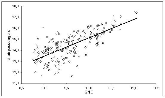
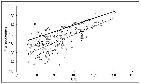
The estimate for the intercept is feature of the function chosen and since the intercept (where C = 0) is outside the data range, the estimated value of α is not of intrinsic empirical interest. The gradient β shows that for every change of unit of business connectivity the unit of airline connectivity is increased by 1.66. The strength of this relationship is given by the correlation coefficient (r) at 0.73 and the coefficient of determination (r 2) at 0.53. The latter indicates that the connectivities account for just above 50% of the variability in passenger numbers across cities. When interpreted in terms of Castells’ spaces of flows, this means that although both layers coincide significantly, there are some important differences in their respective geographies.

These differences can be assessed through an assessment of the differences from the regression line (and therefore the model). Therefore, in addition to statistical results of estimated constants and coefficients, in this study our interest in this model particularly focuses on the residuals. It is these latter that indicate the relative position of a city in the two processes being represented by the variables. For instance, the regression line of the equation is shown in Figure 1 on which the 214 cities are also plotted. By far the largest residual (vertical distance between a point and the regression line) is in the upper left of the diagram. This city has many more visitors than its connectivity predicts – it has one of the lowest connectivities and yet is easily in the top quartile for numbers of visitors. The city is Las Vegas. Although not a major global service centre, it attracts huge numbers of visitors as a global tourist attraction. This is the largest error terms in the model because the premises of the model – that service connectivity on its own or as a surrogate for general business activity – least fit the reality of what attracts air passengers to Las Vegas.

Regression residual analysis is a very powerful tool for understanding processes because it can identify which cases do not fit the model thus indicating, as the Las Vegas example shows, alternative processes to be strongly operating. Thus much of the reporting of results below focuses on residuals. In the results the residuals are reported as standardised measures (in units of their standard deviation from the mean) to aid interpretation. Basically, standardised residuals with values more than 1 or less than -1 suggest the possibility of processes outside the model being important, above 2 or less than -2 strongly suggest this and, above 3 or below –3 definitely indicate the operation of a process not in the model. The largest residual value in our model is Las Vegas with an exceptional 3.24, indicating without doubt the existence of an alternative process. The Las Vegas case is clear-cut which makes it a useful pedagogic example, but other large residuals are less obvious and they are what makes residual analysis more useful and interesting.

Results from a two model analysis

The model specified in equation [4] above has a pedagogic use but it is not the relationship that constitutes the results of this study. On computing the residuals from this model it was found that the US cities values were very unevenly distributed. All US cities had positive residuals: they had more passengers than predicted, which indicates that US cities constitute a different population of cities in terms of the relationship we are modelling. The positive residuals could result from extra air travel amongst US cities or less global service connectivity, a feature of US cities previously reported by Taylor and Lang (2005). In reality it is almost certainly a combination of both US particularities. For this reason we have chosen to carry out two separate regression analyses, one for the 37 US cities in our roster and another for the remaining 177 cities.

The two models are illustrated in Figure 2, which shows the US regression line wholly above that for the rest of the world. These lines represent the following equations:

(i) for US cities

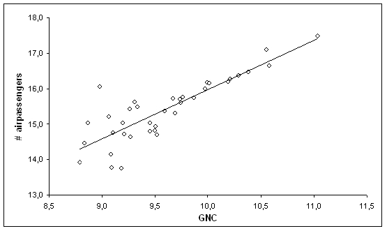
(ii) for non-US cities

Note from equations [5] and [6] that the gradient is smaller for US cities. This means that the rate of increase in connectivity generates a smaller increase in air passengers to US cities than to non-US cities, albeit that the regression line in the data range constantly remains much higher for US cities throughout the entire data range. Put in another way: the decline in passenger numbers from New York as connectivity decreases is smaller than from London, albeit not great enough for the regression lines to cross: the US model always predicts more passengers for a given level of connectivity (Figure 2), an artefact of the well-developed and deregulated airline market in the United States (Doganis, 2001).

As we might expect the coefficients measuring the strength of the relationship are also quite different. For the 37 US cities the correlation coefficient is a very high 0.85 producing a coefficient of determination of 0.73. This indicates that for the USA our model works extremely well; the premise that air passenger numbers can be predicted accurately by connectivity is validated. Of course, the 177 other cities cover a wider range of circumstances and would thus not be expected to have such a strong model relationship. This is the case: the correlation is 0.78 producing a coefficient of determination of 0.61. However, this is still a very good result and again validates the model in general terms.

Residual analysis I : The USA model

We will start with the US model since the results are much simpler. Given this extremely well-fitted model residuals are small with only seven cities with residuals above/below ±1, only two of which are above/below ±2 (Table 1). As well as cities and their residuals, this table suggests basic reasons for the residuals. High residuals can result from the city being either over-visited or under-serviced (or a mixture of both). In Table 1 we have provisionally suggested which interpretation applies to each of the cities. For instance, the city with the largest residual is Las Vegas, which we discussed previously for the combined city model (equation [2]); in this US model the residual is somewhat smaller but still substantial. Honolulu and New Orleans are also clearly tourist destinations that are over-visited relative to their respective service provisions, while the other positive residual suggests a different process outside the model: Phoenix has been notorious for its lower-than-expected rate of services (Short, 2004). The negative residuals cover 4 eastern cities; the two in the north east are industrial cities that we posit to be under-visited; possibly the two south eastern cities are over-serviced ( Charlotte through its banking and Richmond as state capital).

What of the leading US world cities? The seven outstanding top cities (as defined by connectivity, see Taylor and Lang 2005) all fit the model very well (residuals below/above ±0.25, except for Los Angeles) but do provide interesting contrasts (Table 2). Only New York and Los Angeles have positive residuals and can both be interpreted as cities that are much more than global service centres, hence each in their own way being over-visited in this analysis. A negative residual for Washington DC is the surprise here since as capital city it might be expected to be over-visited; however it appears that the quantity of services the political function attracts outweighs the visitors: we interpret the city as over-serviced. Other more ‘specialised’ service cities can be interpreted in the same way: San Francisco for its banking and Miami for its Latin American headquarters are both considered relatively ‘over-serviced’. On the other hand, Chicago and Atlanta’s negative residuals are more likely due to being under-visited (remember airline hub-ness is removed from the data). Of course, these interpretations may be contested but the results do show the potential of residual analysis to throw up interesting questions.

Residual analysis II: The rest of the world model

As the coefficients reported above imply, the non-US city model has a much larger proportion of reasonably high and low residuals: 70 of the 177 cities have residuals above/below ±1. Given that we have separated out the US cities, the question arises whether there are other regions that might be separated from this reduced world model. Table 3 has been constructed to consider this question. Remember that for the original model (equation [4]), all US cities had positive residuals; in Table 3 this range is represented by the first two columns. Clearly no other region has a distribution of residuals as biased as the US had for the initial model: all regions have a reasonable spread of positive and negative residual cities. Certainly differences between regions are not enough to require a further division of our roster and we will proceed with our non-US model.

There are 26 cities with positive residuals above and 34 cities with negative residuals below one (Table 4), which suggests the possibility of processes outside the model being important. The cities thus identified constitute a varied group, and different interpretations can be given for the various residuals. Some of the top cities are capital cities that may be over-visited for their political function and under-serviced because of more important global service centres nearby, for example Toronto for Ottawa and Milan for Rome. In the latter case, since Bologna and Turin both occur in this list Milan’s ‘service shadow effect’ extends beyond the country’s capital. Other ‘second cities’ in the list that may be similarly afflicted are Manchester, Gothenburg and the classic case in service deficiency: Osaka (Hill and Fujita 1995). The negative residual cities in Table 4 that suggest the possibility of processes outside the model being important are more easily interpreted. Hamilton (Bermuda) and Luxembourg City, for instance, are specialist financial centres that can be deemed over-serviced. Another interesting feature of the negative residuals is the appearance of many Eastern European cities. These can be considered to be over-serviced given the attraction of global service firms to post-Cold War Eastern Europe to take advantage of new economic policies, especially the selling of state assets. Cities such as Rotterdam and Antwerp, in turn, are clearly under-visited (through their airports) because both cities are within short railway journeys to alternative large international airports ( Amsterdam and Brussels respectively). An important reason for some of the deviations from the model can therefore be traced back to the fact that airline connectivity does not always assess the connectivity of a single, central location. Rather, some airports are in practice serving city-regions that may consist of one or more major cities together with their hinterlands, thus underestimating the infrastructural connectivity of some secondary cities and overestimating this connectivity of their neighbouring, dominant world city.

Finally what of the leading non-US world cities? Table 5 shows the top ten non-US world cities as defined by service connectivity from the ‘Global North’ plus the top ten of the ‘Global South’. Most show a good fit to the model but there are several moderate exceptions. London and Paris, like New York and Los Angeles before, are much more than global service centres; this is reflected in their sizeable positive residuals interpreted as their being over-visited. In contrast Tokyo’s negative residual suggests it is over-serviced: participation in the Japanese economy still means going through a lot of government channels given a fairly regulated economy. This implies that location in Tokyo is crucial, and results in the city being over-serviced. The Global South cities also exhibit a good fit. The largest positive residual, Bangkok, can be interpreted as over-visited. The four cities with negative residuals are interpreted as over-serviced, albeit for different reasons: Kuala Lumpur and Jakarta are part of a world economic region that is heavily defined by banking and finance services ( Taylor, 2004); Beijing and Shanghai are similar to Eastern European cities for attracting global firms to service their reformed economy.

Conclusion: back to Castells

In this research note we have taken the opportunity of comparing results from two unique data analyses that deal with connectivities between large numbers of cities. This has enabled us to provide some detail about how various cities fare in our model linking measures of inter-city relations in two layers in Castells’ global space of flows. This has produced two distinctive findings: first, the model we propose and calibrate does provide a relative good description of the relationship between the particular spaces of flows, and second, there are numerous explicable divergences from the model. We interpret these as three levels of complexity as follows.

• There is a general overall globalization structure that is a space of flows, which is why the cross-layer model is successful.
• There are multiple globalisations in the various layers of the space of flows, these are the many different processes that constitute the overall structure. We incorporated just two such processes in our model.
• There are a myriad uses of cities in the multiple globalisations, these provide the many roles that cities can play as nodes in the space of flows. This was illustrated by the residual cities in our model.

Castells’ space of flows provides a rich conceptual framework for understanding the spatiality of globalization. We are only just beginning to appreciate the empirical complexity of this socially constructed mega-space.

REFERENCES

Beaverstock, J. V., Smith, R. G., Taylor, P. J, Walker, D. R. F., Lorimer, H., 2000a, Globalization and world cities: some measurement methodologies. Applied Geography, Vol. 20, 43-63.

Beaverstock, J. V., Smith, R. G., Taylor, P. J., 2000b, World city network: a new metageography? Annals of the Association of American Geographers, Vol. 90, 123-134.

Beaverstock, J. V, Hubbard, P. J., Short, J. R., 2004, Getting away with it? Exposing the geographies of the super-rich. Geoforum, Vol. 35, 401–407.

Castells, M., 1996, The Information Age: Economy, Society, and Culture Vol. I – The Rise of the Network Society. Oxford: Blackw ell.

Castells, M., 2001, The Information Age: Economy, Society, and Culture Vol. I – The Rise of the Network Society (2 nd edition). Oxford: Blackw ell.

Choi, J.H., Barnett, G.A., Chon, B.S., 2006, Comparing world city networks: a network analysis of Internet backbone and air transport intercity linkages. Global Networks, Vol. 6, 81-99.

Denstadli, J.M., 2004, Impacts of videoconferencing on business travel: the Norwegian experience. Journal of Air Transport Management, Vol. 10, 371-376.

Derudder, B., 2006, On conceptual confusion in empirical analyses of a transnational urban network. Urban Studies, Vol. 43, 2027-2046.

Derudder, B., Witlox, F., 2005, An appraisal of the use of airline data in assessing the world city network: a research note on data. Urban Studies, Vol. 42, 2371-2388.

Derudder, B., Taylor, P. J., Witlox, F., Catalano, G., 2003, Hierarchical tendencies and regional patterns in the world city network: a global urban analysis of 234 cities. Regional Studies, Vol. 37, 875–886.

Derudder, B., Taylor, P. J., 2005, The cliquishness of world cities. Global Networks, Vol. 5, 71–91.

Derudder, B., Witlox, F., Taylor, P.J., 2007, United States cities in the world city network: comparing their positions using global origins and destinations of airline passengers. Urban Geography, Vol. 28, 74-91.

Doganis, R., 2001, The Airline Business in the 21 st Century. London and New York: Routledge.

Godfrey, B. J., Zhou, Y., 1999, Ranking world cities: multinational corporations and the global urban hierarchy. Urban Geography, Vol. 20, 268-281.

Graham, S., 1999, Global grids of glass. Urban Studies, Vol. 36, 929-949.

Hill, R.C., Fujita, K., 1995, Osaka’s Tokyo problem. International Journal of Urban and Regional Research, Vol. 19, 167-93.

Keeling, D. J., 1995, Transport and the world city paradigm. In P. L. Knox, P. J. Taylor, editors, World Cities in a World-System. Cambridge: Cambridge University Press, 115–131.

Knox, P. L., 1995, World cities and the organization of global space. In R. J. Johnston, P. J. Taylor, M. J. Watts, editors, Geographies of Global Change. Oxford: Blackwell, 232-248.

Miller, W. H., 1999, Airlines take to the internet. Industry Week, Vol. 248 (15), 130–134.

Sassen, S., 1991, The Global City: New York, London, Tokyo. Princeton: Princeton University Press.

Sassen, S., 1998, Globalization and Its Discontents. New York: New press.

Sassen, S., 2001, The Global City: New York, London, Tokyo (2nd edition). Princeton: Princeton University Press.

Shepherd Business Intelligence, 2005, http://www.shepsys.com.

Short, J. R., 2004, Black holes and loose connections in the global urban network. The Professional Geographer, Vol. 56, 295-302.

Smith, D. A., Timberlake, M., 1995a, Cities in global matrices: toward mapping the world-system’s city-system. In P. L. Knox, P. J. Taylor, editors, World Cities in a World-System. Cambridge: Cambridge University Press, 79-97.

Smith, D. A., Timberlake, M., 1995b, Conceptualising and mapping the structure of the world system’s city system. Urban Studies, Vol. 32, 287-302.

Taylor, P. J., 1997, Hierarchical tendencies amongst world cities: a global research proposal. Cities: The International Journal of Urban Policy and Planning, Vol. 14, 323-332.

Taylor, P. J., 1999, So-called “world cities”: the evidential structure within a literature. Environment and Planning A, Vol. 31, 1901-1904.

Taylor, P. J., 2000, World cities and territorial states under conditions of contemporary globalization. Political Geography, 19, 5-32.

Taylor, P. J., 2001, Specification of the world city network. Geographical Analysis , Vol. 33, 181-194.

Taylor , P. J., Catalano, G., Walker, D. R. F., 2002a, Measurement of the world city network. Urban Studies, Vol. 39, 2367-2376.

Taylor, P. J., Catalano, G., Walker, D. R. F., 2002b, Exploratory analysis of the world city network Urban Studies, Vol. 39, 2377-2394.

Taylor, P. J., Catalano, G., Gane, N., 2003, A geography of global change: cities and services, 2000-01. Urban Geography , Vol. 24, 431-441.

Taylor, P. J., 2004, World City Network: A Global Urban Analysis. London: Routledge.

Taylor, P. J., Lang, R. E., 2005, U.S. Cities in the ‘ World City Network’. Washington, DC: The Brookings Institution.

Table 1: High and low residual US cities.

Table 2: Leading US world cities

Table 3: Frequencies of residuals by world regions.

* All but two are Canadian cities, whereby the two non-Canadian cities ( Nassau on the Cayman Islands and in Hamilton on Bermuda) have negative residuals. Thus 5 of Canada’s 7 cities are in the first two columns ( Montreal and Ottawa are in the penultimate column), which implies that Canadian cities may be more like US cities than the rest of the world.

Table 4: Extreme residual non-US cities.

Table 5: Leading Non-US world cities, North and South.

Figure 1: Regression analysis for 214 cities

Figure 2: The two models

Figure 3: Regression analysis for US cities (model 1)

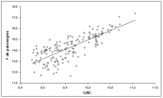Figure 4: Regression analysis for non-US cities (model 2)

NOTES

* Peter J. Taylor, Department of Geography, Loughborough University, E-mail: p.j.taylor@lboro.ac.uk

**Ben Derudder, Department of Geography, Ghent University, E-mail: ben.derudder@ugent.be

***Frank Witlox, Department of Geography, Ghent University, E-mail: frank.witlox@ugent.be

1. We would like to thank Bob Lake and one of the anonymous referees for their useful comments on an earlier draft of this paper. This research has, in part, been funded by the Scientific Research Fund-Flanders, Research Project G.0214.04.

2. The hypothesis that the dramatic increase of ICT-enabled business practices actually boasts corporeal travel and associated face-to-face contacts has recently been supported by Denstadli (2004). Denstadli’s analysis suggests, for instance, that videoconferencing goes hand in hand with business air travel, with substitution rates as low as 2.5–3.5%. Thus ICT-practices pose no serious threat to the airline industry, and should be regarded as supplementary to personal contact. However, this does not imply that there is a direct parallel between the geographic structure of, say, the Internet backbone and air transport networks. Choi et al. (2006), for instance, have shown that both ‘spaces of flows’ are similar, but by no means exact copies. Both structures exhibit strong inter - link a ges between North American and European cities, and feature the London–NewYork dyad as the strongest linkage in the global flow of information and peopl e . But differences between the two networks do exist. For instance, Asian cities have lower positions in the Internet network than in the air transportation n etwork, which reflects a relatively weak deployment of inter- and intra-regional backbone connections.

Note: This Research Bulletin has been published in Urban Geography, 28 (3), (2007), 232-248