GaWC Research Bulletin 24

The analysis of cities and urban agglomeration began with the seminal works of von Thünen (1826), Weber (1909), Christaller (1933), Lösch (1940), who explained that urban agglomeration is a scale economies process. A brief historical overview of this discipline take us to analyse the initial studies by Adam Smith (1776) about labour division and specialisation. Marshall (1890) already started the first contribution to industrial allocation, explaining the benefits of agglomeration through externalities. Advantages of agglomeration explain the city genesis. These advantages increase as growing and specialisation do, but they become a problem when the urban structure grows too much and congestion costs are too large.

In the first part of the 20^th, Christaller (1933) offered an interesting regional location analysis based on the Central Place Theory. He introduced concepts such as city systems, and urban hierarchy, usual terms in today research papers. Completing this model, Lösch (1940) proves that under certain conditions the obtained equilibrium results in a hexagonal morphology of city systems.

After some empirical analysis, Zipf (1949) discovered there is a regular distribution of the sizes of the cities of a country directly related to -as a sequence- the importance of each one of them in terms of population. This particular case of rank-size distribution is called Zipf law (ZL).

Isard (1956) renewed urban economics translating and systematically exposing texts from the German School. It was not until the pioneering model of Alonso (1964) when urban economics took off. This model supposed the first theoretical analysis, under a standard microeconomic framework, where residential choices of urban inhabitants are studied. This model was generalised later on by Mills (1967), Muth (1969), De Salvo (1977), Fujita (1989) and others. Besides Zipf (1949) research and ZL suppose an empirical evidence for many different countries.

Mainly, there are two theoretical arguments for explaining ZL. First, Krugman (1991) did an analysis of urban agglomeration through a simple model of two regions. However, his general equilibrium framework is useless for explaining ZL because the model outcome was a set of identical (in terms of size) cities or just one city. New generalisations of this model - where congestion and spillovers (of information) are included- are able to generate rank-size distributions (see Alonso-Villar, 1996; Brakmant et al., 1999).

Second, according to Simon (1955) arguments on lognormal distributions, Berry (1961) exposed that lognormal distributions (as terminal points of random pertubances) reach higher degree of entropy (level of misinformation). Gabaix (1999a, 1999b) revisits original arguments of Gibrat (if growth process is stationary, distribution of cities will follow the ZL) in his late papers.

The target of this paper is to analyse the process of agglomeration of Spanish regions in the last 50 years, using the estimation of rank-size equation. The second epigraph is dedicated to theoretical framework. The sample, method and some considerations are performed in the third. Results are analysed in the fourth section. The fifth concludes. .

THEORETICAL BACKGROUND

Zipf Law

Zipf described the process of agglomeration, there are two forces implied in the growth and development of cities. "Unification" force, derived from specialisation and industrialisation of cities (circular causation for Myrdal, 1957, and Hisrchman, 1958), implies large processes of agglomeration and consequently big cities. "Diversification" force, driven by commuting cost (the distance between raw materials location and the cities itself), could be the reason for a dispersed habitat.

Following Zipf arguments, an increase in labour productivity (or a decrease in commuting cost) produces higher unification force and, therefore, a smaller set of bigger cities. If cost decreases (or productivity grows) indefinitely, the only outcome should be an extreme situation: a large city, where the whole population lives (identical result than Krugman, 1991). In this sense, urban agglomeration is caused by technology (in terms of productivity or commuting).

However, since is not possible to allocate all the population in only one city (maximum level of agglomeration) or in n-identical cities (absolute spreading) the distribution of population will depend on the intensity of each force, and the outcome will be an equilibrium between them.

A rank (r) (that follow the next specification) is obtained after ordering the cities in term of its population:

where r is the position of the city in the rank; q is the result of unification and diversification forces; P_j is the population of each j-city; and K is a constant.

In equilibrium context (under Zipf hypotheses), where both forces are balanced the value of q should be one. Then, ZL can be defined as:

where R_j is the rank of the j-th city, S_j is its size (population) and C is a constant.

Then, ZL is only a particular case of Lotka equation. We may conclude that ZL expresses the rank of cities in terms of their population, where the largest one has rank 1, the second city holds the 2^nd position, and so on. Under ZL (q=1) the most populated city will be k-times larger than the k-th city.

The empirical test of ZL can be fulfilled through the estimation -in log form- of [3], in which the value of q² is derived,

being j=1,2,...n, the number of cities. In terms of distribution, this means that the probability of the size of any city being larger than any T is to 1/T: P(Size>T)= α /T^q_, with q≅1, i.e. LZ³.

When q>1, the largest city is bigger than ZL forecast, so there is an inequality in terms of city sizes, where the biggest one is more populated than ZL prediction. If 0<q<1, the function gradient is smaller that ZL prediction, resulting in a more homogeneous distribution of cities. However, small values of q (q<0.7) imply a big degree of dispersion (urban sprawl).

Zipf Law in General Equilibrium Framework

Krugman (1991) begun a new research line, revisiting the classical Germans works, specially the contributions of Myrdal (1957) and Hisrchman (1958). He avoided the idea of perfect competition using monopolistic competition framework; where scale returns are produced at firm level⁴. Nevertheless his model is useless for explaining rank-size distribution because the model outcome is just one city or n-identical cities (spreading)⁵. If nominal wages are higher in large cities, labours move to big cities, causing higher economic growth (demand increases → bigger production higher → labour demand, etc.) - "forward linkage". As a consequence of a larger local market, new scale returns are produced, so the process will be more intense - "backward linkage". In the long term, a complete agglomeration will be produced.

The non-existence of congestion in this model drives to the result mentioned above, where rank-size distribution can not be analysed. However, new papers introduce congestion in this framework. Congestion is a consequence of urban agglomeration (increasing with the city size). Usually, two types of congestion costs are analysed in the literature: commuting and congestion costs, assuming that they limit the growth of cities: (a) commuting costs are generally compensated with lower housing prices (Krugman y Livas Elizondo, 1996)⁶. (b) costs produced by agglomeration: crime, pollution, traffic, etc. Alonso-Villar (1996) explains this cost introducing an "iceberg" parameter that affects negatively the labour supply. Thus, commuters (in the case of Krugman-L.Elizondo) suffer high commuting costs and central householders (A-Villar frame) bare high levels of crime, noise, etc., measured in high prices. However, Alonso-Villar offers an alternative: if commuting costs are too high, householders could choose a location outside the city-core -avoiding congestion- generating a more dispersed habitat. Puga y Venables (1997) introduced the vertical relationship between firms as another alternative: if commuting costs (related to purchase of intermediate commodities) are too high, firms have incentive to change their location.

Despite these references (and improvements in location theory), one of the main features of increasing return models is that equilibria are not unique and un-predicted. Rauch (1993) and Arthur (1990) described that the final equilibrium reached by a region is conditioned by its history. Moreover, the role of its history is not clear, the final outcome could not be related to its the origin but caused by any historical accident ("big-push"), being this the only responsible for the final equilibrium.

The last generation of these models introduce human capital. This variable is analysed as an externality that arises from the interaction between individuals ("informational spillover"), reinforcing agglomeration processes. This positive local externality causes an increase in labour productivity and stimulates the development of the city. The whole process repeats itself through "forward" and "backward" linkage. The most important consequence of this model is that it determines a new kind of equilibrium: co-existence of two kind of cities, big and small ones. Brakman et al. (1999) generalised that idea in a N-cities model, using iceberg costs, technological spillovers and congestion. Labour migration is produced until real wages between cities is balanced, resulting in an equilibrium where city-sizes are not identical. The final distribution is a consequence of the history ("path-dependent"), where congestion ("negative feedbacks") is determinant in the final location of firms.

As a conclusion, last papers show that rank-size distribution is perfectly compatible with general equilibrium modelling. So, ZL could be the outcome of any particular modelling.

Profits and Costs of Agglomeration

It is common in recent literature to detail the high cost of agglomerating (in terms of noise, pollution, commuting and so on), but also there many benefits in this process. Along this section main benefit/cost and contribution are briefly explored.

b) Moving people. "Economics of superstars" (Rosen, 1981) is an easy way of explaining this advantage. The market for any professionals is larger in a big city (than in a village) and their chances of matching are also higher. That is why skilled workers usually migrate to big cities⁷, even unskilled have more opportunities in cities^{8, 9}. A larger labour market is another advantage of urban agglomeration. Similar arguments are related to the bargaining power of urban workers, an utility derived from human interaction and a lower risk of unemployment. (Rosen, 1981; Lucas, 1988; David y Rosembloom, 1990; Rauch, 1991).

c) Informational spillovers and "learning in cities". Intellectual atmospheres are common in big cities, the concentration of skilled workers arises to an informational spillover over all labours (Jacobs, 1969; Lucas, 1988; Saxenian 1994). Some recent papers connect firms' concentration, intellectual spillovers (education) and economic growth (Benabou, 1993; Rauch, 1993; Martin y Rogers, 1994; Henderson, Kuncuro and Turner, 1995).

a) Costs of living and commuting. Both are clearly correlated to city size. A bigger city means higher costs of living and commuting. These costs are arguments against urban agglomeration and metropolitan areas. (Henderson, 1974; Glaesser, 1998).

b) Pollution. This is not just an urban problem, but it is frequently related with the size of the city (emissions). Kahn (1996) shows that this problem is presently decreasing because of technology and, specially, governmental legislation.

c) Other costs. Another kind of common problems at the cities are high rates of crime (Rosen, 1981), adverse selection and presence of free-riders (Becker, 1968; Glaeser, 1998), and are caused by the anonymity.

METHODS, DATA AND SAMPLE

Source. The Statistical Information Section of the National Institute of Statistics (Instituto Nacional de Estadística, NE) provided us the population database. This information is available for all administrative urban nucleus, without any cut-off. The periodicity is every ten years data. The sample used in this paper cover the available information since 960 thru 1998.

A secondary analysis was performed using information supported by BBV (stock of public and private capital; gross added values series -by sectors). Even the Encuesta de Población Activa has been study for analysing labour productivity (in industrial sector).

Method. Estimation of distinct values of q from equation [3] -in logarithmic specification [4]- is performed by OLS. Sample minimal size (S_min=10.000) is cities of at least ten thousand people, following Brakman et al. (1999) criteria. Similar estimations are repeated using a larger sample (S_min=5.000) for a better understanding of urban agglomeration processes.

Sample (cut off =S_min). The size of the last city (included in the sample) is determinant in analysing rank-size distribution. Different authors have used several samples. Gabaix (1999b) proposed to use a sample of the 100 largest cities. Zipf (1949) also used the same cut-off. (100 largest American metropolis) although, afterwards, he used open samples (S_min=50.000). The analysis of Mills & Hamilton (1994) is done for 2.500 people cities (cut-off). Brakman et al. (1999), used S_min=10.000 habitants nucleus in Holland.

RESULTS

Along this section we will perform the estimation of rank-size equation [4]. This estimation has been made for each region for all the periods (1960-1998). Thus we have five estimated equations for each region. The outcome of this analysis is shown in the table below.

Table 1: for each region

We will analyse these values in three steps. First, several paths of urban agglomeration are observed: a very few regions are in process of agglomeration, others in stability and the most of them are in process of sprawling. Second, different economic arguments (scale economies, path dependence, stock of capital, etc.) are used for a better understanding of these stylised facts. Finally, the path of migration is contrasted; we will use a bigger sample (and the equation above is re-estimated for all the cases).

Four Phases of Urban Agglomeration in Spanish Regions

A simple view of table 1 reflects that, along the time, some regions have been showing processes of agglomeration (Asturias, Castilla la Mancha (CLM) and Navarra); other regions (Baleares, Cataluña, Cantabria and Madrid) have been diminishing their level of agglomeration during the whole period. A third group (Andalucía, Aragón, País Vasco and Valencia) show an irregular behaviour: their levels increase sometimes and decrease some other timer (we will name them "stable"). The last group contains regions (Canarias, Castilla León, Extremadura, Galicia and Murcia) that, during the period, achieve the top level (maximum level of agglomeration) and afterwards beginning to invert this process, i.e. there is an inflexion point. Table attempts to summarise these scenarios.

Table 2: Phase of agglomeration of Spanish regions

Regions in group D, are decreasing their level of agglomeration during the whole period (thus, they suffer from congestion¹⁰); group A includes regions in phase of constant unification (agglomeration becomes stronger without congestion); group I includes regions with one inflexion point; the last group regions with more than one inflexion point or stables are presented.

About these results, three stylised facts seem to be relevant:

1. In 1998 (right side, table 2), still there are a few Spanish regions with very high level of agglomeration (Asturias, Cantabria, Madrid, Navarra and so on).

2. Most Spanish regions have reached their maximum level of agglomeration before 1960 or between 1960-1998. After that point of inflexion they began to present congestion in their urban structures.

3. Other group -Valencia or Andalucía- presents not clear process of agglomeration neither congestion for the whole period. Cities are unevenly set across the space, not presenting any system of cities.

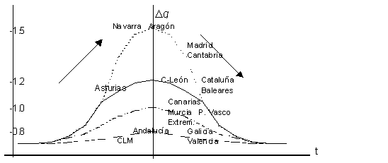
Some Economic Explanations

Urban agglomeration is the result of processes of scale economies (forward linkage) and increasing local market size (backward linkage). Although there is an upper limit for this process: the appearing of congestion. Three important arguments (labour productivity, path dependence and stock of capital) for explaining the processes of agglomeration/congestion of Spanish regions will be used below.

1. An increasing level of labour productivity (in industrial sector) is one of the main arguments for explaining scale economies in urban agglomeration. Usually, informational spillovers, decreasing costs, specialisation, etc. are different advantages of agglomerating. On the other hand, noise, commuting, crime, and so on, are disadvantages that explain low levels of productivity (and the presence of congestion in the city).

During the period 1980-1998¹¹, the regions with a higher variation of labour productivity with respect to national average (μ =3.19) were¹²: Extremadura, País Vasco, Galicia, Navarra and Aragón. The first three have never been very agglomerated (q≅1) and the other regions do not present congestion.

On the average we find C. León, CLM and Asturias. C. León is on the inflexion point, so it does not present too much congestion; CLM and Asturias are still in phase of agglomeration.

The remaining regions are below average. Baleares, Cataluña, Cantabria, Madrid reached high levels of agglomeration in the past, and now are in phase of congestion. Therefore, the results are those expected.

Andalucía and Valencia have a very low level of agglomeration (and congestion) but they have not a high level of industrial labour productivity. We have no explanation for that.

According to these results, we may conclude that it seems to be a relationship between industrial labour productivity and the level of congestion in urban agglomeration. As we supposed at the beginning, this relationship is indirectly proportional.

2. Another argument for explaining the present level of agglomeration is the dependence of the past (Brakman et al., 1999). The existence of congestion is the consequence (not the cause) of any previous process of agglomeration. Regions with initial very high values of agglomeration are determined to present congestion. In this sense we say they are path dependent. On the contrary a region featured by "urban sprawl" should not present congestion.

The regions with a higher starting point (see table 2) are, in this order, Madrid, Cantabria, Aragón and Cataluña. With the exception of Aragón (it is quite irregular, sometime it rises and other times falls) all of them are in clear process of dispersion. Regions with a low start point (in this order, CLM, Extremadura, Andalucía and Galicia) present agglomeration until 1990, after that they remain stable or present a very slow inflexion; moreover, CLM is still growing. With q<1, in 1960, Valencia and Asturias do not present congestion.

Regions beginning with q≅1 in 1960 do not show an inflexion point until the 80's (Canarias and Murcia) or the 90's (C. León), while País Vasco remains stable. Baleares has a starting point of 1.06 and is decreasing during the whole period. Navarra seems to be an exception but the estimation of q for 1960-70 is not significant.

Then, the idea of dependence of the past in the process of agglomeration seems to be confirmed in the Spanish case. The stylised facts shown here reveal an inverted U curve. This curve is the temporal path of urban agglomeration. As shown below (figure 1) this curve's shape is concave. The process of agglomeration is: it increases (q>0, q' <0), defines a maximum (q'=0), and begins to spread (q<0, q' >0).

In figure 1, several temporal paths of agglomeration of Spanish regions (during the period analysed) are presented. Regions allocated at the left side are increasing their level of agglomeration; on the axis, are those regions with stabilised process. In the right side, regions in phase of spreading are shown.

Figure 1: Temporal paths of urban agglomeration

The different lines represent several process of agglomeration and there are various values of q that define a maximum. Then, regions reach their the upper limit (inflexion point) for distinct values of q.

Madrid (D), Aragón (S), Navarra (A) and Cantabria (D) are in the first group. The main feature of this path of growth is a very high level of agglomeration (q takes a value higher than 1.4) in the present or in the past time.

In a second group there are regions that reach -or have reached- values of q close to 1.2, like Cataluña (D), Baleares (D) or C. León (I). Asturias (A) seems to belong to this group. The regions allocated in the third group reach values of q close to one, as País Vasco (S), Canarias (I), Murcia (I) and Extremadura (I). Finally, with q<1, regions present "urban sprawling", like CLM (A), Andalucía (S), Galicia (I) and Valencia (S).

With this information we can conclude that, for the case of Spanish regions, there are several values of q that define a maximum. Therefore, there are different patterns of urban agglomeration in Spain.

where k^* are regional border.

When decreasing commuting costs make them an irrelevant part of the household budget (transportation costs are not determinant in maximisation consumer problem of allocation), a dispersed habitat could be a solution in equilibrium (Alonso-Villar, 1996)¹³. In any case, the area of influence of any metropolis becomes larger if commuting cost falls, therefore the level of congestion also decreases.

Using the available information (see appendix) of the variation rate of public and private capital for the Spanish regions, at the aggregate level, in the period 1981-1995, we get the next ideas.

1. Variation of public stock of capital (national average, μ =2.65). Galicia, Extremadura, Navarra, Murcia, Cantabria, País Vasco, Andalucía and Baleares are on top; Asturias, Cataluña and Valencia on the average; the remaining regions are under the average level.

2. Variation of private stock of capital (national average, μ =1.4). Canarias, Murcia, Baleares, CLM, Andalucía and Valencia are on top. Navarra, Madrid and Aragón on the average level.

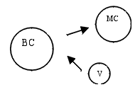
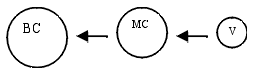
These results seem to indicate that there is not any clear relationship between aggregate stock of capital and the level of agglomeration.

Re-estimation of [4] for S_min=5000 habitants

Along this sub-section the estimation of [4] is repeated again; however, a bigger sample is used, in which smaller cities are included (lower-limit is 5,000 habitants in contrast of 10,000 habitants). Table 3 summarises the whole analysis. For a deeper analysis of these results, we will study the regions using the group classification described above (table 2). For a better understanding we will label "village" (V) to small cities, "medium cities" (MC) to the regular-size cities, and "big cities" (BC) to these specific kind.

Group "D" (Baleares, Cantabria, Cataluña and Madrid). Since 60's till 80's (Baleares until 90's) all this regions are in process of agglomeration and, after 80's begin to show congestion. If we put together results shown in table 1, 2 and 3 we got the next explanation. Table 1 shows that all these regions are in phase of spreading but in table 3 we find agglomeration.

Table 3: for each region (S_min=5,000 hab.)

All the coefficients are significant for α =0.01, except * α =0.05 and ** α =0.10. Where (----) means not significant coefficient. Once again, La Rioja results not significant, so is not analysed.

Our view is that during the whole period, people have left the big cities looking for new residential places in medium cities (spreading), because of congestion. However, people who were living in "villages" also left their small cities and moved to big cities (agglomeration). With both sample (10,000 and 5,000 hab.) we can capture both processes. Then, since 60's thru 80's urban inhabitants moved to medium cities and rural ones went to big cities. After 80's, big cities and also medium cities suffered high problems of congestion and, therefore, people moved to villages again (spreading in both samples).

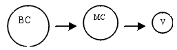
Group "A" (Asturias, CLM and Navarra). If we compare table 1 and 3 we still find processes of agglomeration in this set of regions. However, we can see that the level of agglomeration is quite lower than those preceding. In this sense, our interpretation is that people live in big cities or villages, nor in medium cities, as we show below.

Group "I". Canarias, C. León, Murcia and Extremadura show very similar behaviour to A. However, Galicia is still in agglomeration (so it is different than in table 1), then Galicia shows another path of population moving, like this.

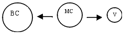
Group "S". Valencia, P. Vasco and Valencia show an analogous process in table 2. Since 80's thru 98's the pattern is very similar to diagram 2. As a result, the distribution in year 2000 is more regular than in 1980. However, Andalucia is different, showing agglomeration during the whole period, so the pattern is similar to diagram 1.

This second analysis with a bigger sample (a smaller cut-off) shows again several patterns of urban agglomeration. Then, our hypothesis of different paths of agglomeration in Spanish regions seems to be also confirmed.

CONCLUSIONS

Along this paper, recent patterns of urban agglomeration in the Spanish regions (1960-1998) have been analysed. To complete this, two different samples have been used. First, a sample where the cut-off was 10,000 inhabitant cities; second, a bigger one, including 5,000 people cities. The main results of the paper are. A) We find several process of agglomeration in Spanish regions. B) The agglomeration process is path dependent. C) There is any relation between labour productivity and pattern of agglomeration. D) In many Spanish regions congestion has been responsible for the present urban sprawl.