GaWC Research Bulletin 199

This Research Bulletin has been published in P Hall and K Pain (eds) (2006) The Polycentric Metropolis: Learning from Mega-City Regions in Europe London: Earthscan, pp. 53-64.

Please refer to the published version when quoting the paper.

(Z)

Organization of the Polycentric Metropolis: Corporate Structures and Networks

P.J. Taylor, D. Evans and K. Pain

 

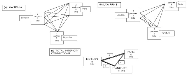
We now start to tackle the central research question: how to capture and measure the ‘space of flows’ in an economy based on knowledge-intensive advanced producer services (APS)? How exactly does information flow from individual to individual, within businesses or organizations, and between those businesses and organizations? How do these flows operate at different geographical scales – within functional urban regions (FURs), between FURs within a mega-city region (MCR), between a group of MCRs such as the eight we have identified for study in North West Europe, and between those MCRs and the rest of the world?

Chapter 2 ended by establishing some preliminary comparative measurements for each region of its polycentricity, as measured by daily commuting patterns. But these, it explained, were in some important sense inadequate: they failed to capture a key element, which was the exchange of information within regions and also between them. In Part 2, we successively seek to establish better ways of measuring these linkages.

This is no easy task. Ideally, we would try to capture the flows directly: by measuring the location of face-toface business meetings, the origins and destinations of telephone calls and email traffic. But, as explained in Chapter 1, data on these flows are sparse and difficult to obtain. In order to approach the problem, we need to reinforce these thin pickings, by going a different way via a less direct route.

As explained in Chapter 1, POLYNET was designed to bring together four sets of conceptual insights: Friedmann’s ‘global city hierarchy’, Taylor’s ‘world city network’, Scott’s ‘global city regions’ and Castells’s ‘space of flows’. The research reported in this chapter brings together these four theoretical approaches. Using methodologies developed by the Loughborough Globalization and World Cities (GaWC) group, we describe and analyse global, European, national and regional spaces of flows through measures of inter-city relations.

Introducing the analysis

We wish to understand how cities and MCRs are knitted together through business practices. In particular, we are interested in business projects that require information and knowledge in several places to achieve their goals. For instance, a law firm may use partners and junior lawyers in several offices to draw up a particularly complex contract for a major client. Such use of a geographical spread of professional expertise is quite common in advanced financial, professional and creative services for large business clients. Thus providers of such services invariably have large office networks in cities and throughout MCRs. Such services are quintessentially city-based economic activities: therefore one important way in which the cities and MCRs are integrated into ‘economic wholes’ is through advanced service provision by firms that are simultaneously local, national and global.

However, one of the most frustrating problems for understanding how businesses use cities and MCRs is the lack of data. In the production of advanced services for business we know that there are numerous communications – face-to-face, telephone, fax and email – but there is no readily available information on these practices. Collecting such information is costly, time-consuming, and rarely very comprehensive. Is there a simpler way to estimate such connections through which service firms link cities and MCRs? We need a surrogate measure using information that is readily available. Well, we can easily find out where offices of service firms are located (e.g. from their websites) and, in addition, the functions and importance of different offices can be gleaned from the available information. With a little simple modelling based upon plausible assumptions, such information allows us to estimate links between cities and the importance of a city in terms of links, which we term its ‘network connectivity’.

A basic example will clarify the method. The office networks of two hypothetical law firms are shown in Table 3.1. Both have just three offices, one each in Frankfurt, London and Paris. The importance of the office is given by the number of partners located in an office – partners are the basic cost centres of legal work. The law firms are similar in size – Law Firm A has six partners and Law Firm B has five partners – but the distributions of partners across the three cities are very different. The largest office is Law Firm A’s in London. We will assume that each partner generates approximately the same amount of business: thus summing the rows for each city measures the amount of law business done in each city. We call this a city’s ‘nodal size’ in Table 3.1 and we can see that London is the leading ‘law city’ in this example, with Frankfurt and Paris ranked second equal.

Table 3.1 The office networks of two law firms

Notes: a Number of partners in the city.
b Number of inter-city partner dyads involving the city (counted on Figure 3.1).

We can go a crucial stage further through the reasonable surmise that links between offices are a simple function of the amount of business done in offices (i.e. the number of partners located there). This is illustrated in Figure 3.1. In Law Firm A, Paris has two partners and Frankfurt only one, therefore there are only two potential inter-partner links. In contrast, London has three partners and therefore there are six potential inter-partner links with Paris and three with Frankfurt. Law Firm B is similarly depicted in Figure 3.1; this time it is Paris that is weakly linked to the other two cities. The key point is that by adding up the links between cities estimates of inter-city connections are derived: Figure 3.1c shows that London–Paris is the strongest link and Frankfurt–Paris the weakest. In addition, all of a city’s links can be added together to indicate the total intercity connectivity of the city. In this case, London is again ranked first (Table 3.1). However, notice that with this measure Paris is more important (has more links) than Frankfurt. It is this latter measure – inter-city network connectivity – that is preferred over simple nodal size as an index of a city’s importance because it tells us how significant the city is across the network.

Figure 3.1 Illustration of inter-partner connections of two law firms

All the results reported in this chapter involve intercity connections of pairs of cities and the network connectivities of cities. The only practical difference is that we use many more firms and cities. It is particularly important to use large numbers of firms so that the idiosyncrasies of individual firms are ironed out in the aggregate results to provide stable, replicable, estimates of linkages and connectivities. While these are based on information about connectivities within individual firms, the inclusion of a large number of firms operating across the cities – as in the very complex Figure 3.1c – can provide vital evidence of potential inter-city network connectivities that are conferred on cities by networks of firms.

Collecting the data

The data collection for this analysis is the largest of its kind ever attempted. Eight service sectors were selected for study: accountancy, advertising, banking/finance, design consultancy, insurance, law, logistic services and management consultancy/IT. Data were collected for the office networks of a total of 1963 firms within the eight MCRs. Sources used varied between countries and included:

• National databases, e.g. Trends-Tendance in Belgium, Hoppenstedt in Germany
• Other directories, Yellow Pages and similar.

There were many examples of firms offering services in more than one sector; in each case the firm’s core activity was identified and it was allocated accordingly. Although not necessarily comprehensive for all city regions, this exercise produced a universe of firms representing a wide range of business services for each region that was in every case large enough for the study.

Each regional team selected firms from their universe of firms for inclusion in the analysis. Firms were chosen both on the basis of local knowledge and for pragmatic reasons. First, firms had to be multilocational, in the sense of having offices in at least two cities. Firms were also chosen on the basis of the quality of information available about them, and ease of obtaining it (e.g. whether a firm had an informative website). Overall the choice of firms had to correspond roughly to the relative importance of different sectors in that particular city region. All these were regional team decisions because each case study is about a distinctive, particular city region. Table 3.2 shows the different numbers of firms sampled by sectors and selected by each team. Each team carried out checks to ensure that variations in the sample shares broadly matched the structure of the sectors in each city region. In cases of a large sample in a specific sector there are no implications for the connectivity and linkage scores obtained.

Table 3.2 Distribution of firms studied in MCRs by sector

The office networks extended to national, European and global scales but here we concentrate on cities and towns within the MCRs. Table 3.3 shows the numbers of firms and cities/towns studied in each MCR. Each regional team selected the urban centres that they thought were important to an understanding of the operation of their city region – it is these cities that are the focus of the research. Again this relied upon local knowledge. Table 3.4 shows detail for the regional cities selected by each team. These cities were used to define city-regional servicing strategies by firms and the regional connectivities for regional cities.

In addition each team selected major national cities beyond their region that they thought were important for understanding their city region. The two German teams coordinated their national city selections to produce a common set. The Belgian team did not select a separate national set of cities because the Central Belgium city region included all major Belgian cities. Table 3.4 also shows the different numbers of national cities selected by each team. These cities were used to define national servicing strategies by firms and the national connectivities for regional cities.

Table 3.3 Data production: Service firms and cities/towns across the MCRs

Table 3.4 Cities chosen for study by mega-city region

At the European and global scales, the cities selected were necessarily were the same for all teams. Based upon previous GaWC analyses of global connectivities (Taylor, 2004a), 25 European top cities were identified: London, Paris, Milan, Madrid, Amsterdam, Frankfurt, Brussels, Zürich, as above, plus Stockholm, Prague, Dublin, Barcelona, Moscow, Istanbul, Vienna, Warsaw, Lisbon, Copenhagen, Budapest, Hamburg, Munich, Düsseldorf, Berlin, Rome, and Athens. These cities were used to define European servicing strategies by firms and the European connectivities for regional cities.

Global-level cities were similarly selected. Based upon previous GaWC analyses of global connectivities (Taylor, 2004a), 25 top world cities were chosen: London, New York, Hong Kong, Paris, Tokyo, Singapore, Chicago, Milan, Los Angeles, Toronto, Madrid, Amsterdam, Sydney, Frankfurt, Brussels, Sao Paulo, San Francisco, Mexico City, Zürich, Taipei, Mumbai, Jakarta, Buenos Aires, Melbourne, Miami. These cities were used to define global servicing strategies and the global connectivities for regional cities.

Unsurprisingly, eight of the global level cities also appear in the European list. Likewise, some European cities will appear in national city lists, and some major national cities in regional city lists. Thus analyses at each different scale will not produce independent measures. This is not a problem because cities by their very nature are multi-scalar in their reach: London, Paris and other cities are simultaneously regional, national, European, and global service centres. However, it is useful that overlaps between scales generally involve less than one-third of cities in any list, allowing distinctive differences across scales to be measured.

Analysing the data: The services activity matrix

These selected firms and cities set the dimensions of the services activity matrix that must be constructed. Because cities are related to four different geographical scales, the overall matrix can be divided into four service activity sub-matrices for the computation of connectivities at different scales. The same rules for allocating service values were adopted across all scales.

To define service values, only two types of information were gathered:

• indications of size of a presence in a city (e.g. number of practitioners or partners working in an office);
• any indications that an office carries out extra-local functions for the firm (e.g. headquarters, research).

Because the form of the information gathered is unique to each firm, it had to be converted into a common data matrix to make comparisons of service values across firms (and therefore all analyses) possible.

The data collected consisted of estimates of the importance of each city or town to the office network of a given firm. The scale ranged from 5 indicating the headquarter location of the firm, to 0 for a city/town where the firm had no office at all. From these data four matrices arraying firms against cities/towns at different scales were produced for each MCR. For instance, for the Randstad the four matrices arrayed the 176 firms as follows: at the city region scale the matrix was 176 firms x 12 cities/towns (see Table 3.3); at the national scale an additional 12 cities were added (see Table 3.4) to produce a 176 x 24 matrix; at the European scale 24 cities (not 25 because Amsterdam was already in the matrix from the regional level) were added for the regional scale) to produce a 176 x 36 matrix; and, at the global scale 24 cities were similarly added (again without double counting Amsterdam) to produce the final 176 x 36 matrix. Each of these matrices is the equivalent to the simple 2 law firms x 3 cities matrix of Table 3.1, except they are very much larger! However the same principles apply for calculating inter-city/town links and city/town network connectivities although they can no longer all be shown as was the case in Figure 3.1. Here it is assumed that the more important the office, the more business will be conducted in that city/town and therefore more information will flow to and from other cities/towns. In other words we can compute the network connectivity of each city/town within its respective MCR. These are the results we now report upon.

Connectivities within North West European mega-city regions

The findings reported in this section are network connectivities, showing connectivity within each MCR as in the final column of Table 3.1. However, because of the large numbers of links involved due to the quantity of data used, all connectivities have been converted into percentages of the most linked city in the respective regions. This also facilitates easy comparison between regions. The results for top six cities/towns in each of the eight MCRs are shown in Table 3.5. The percentages in this table can be interpreted as follows. Taking the first case as the example, it is clear that in the Randstad MCR, Amsterdam and Rotterdam are by far the most connected cities: very many service firms do important business in both cities thereby connecting them to the rest of the region. Utrecht and The Hague are quite well connected, whereas the network connectivities of Alkmaar and Amersfoort are relatively low. Thus, a clear pattern of network connectivities is shown, dividing the cities/towns into three pairs.

Table 3.5 Network connectivities within MCRs

The eight MCRs fall into two groups: four ‘primate’ regions and four regions with more complex patterns. Clearly Dublin, Frankfurt, London and Paris strongly dominate the intra-regional linkages in their respective regions. Three regions show a duopoly of linkage dominance with Rotterdam rivalling Amsterdam, Antwerp rivalling Brussels, and Basel rivalling Zürich. In the first we have previously noted that Utrecht and The Hague are also relatively important but there are no equivalent ‘medium-high’ linked cities in the other two regions. However, in the final region, RhineRuhr, the situation is an enhanced version of the Amsterdam situation with all six cities showing relatively high levels of connectivity and Düsseldorf and Cologne almost tying for first place.

These initial results show a clear ordering of multi-nodality in North West European MCRs: RhineRuhr, the Randstad, Central Belgium, EMR Northern Switzerland, Rhine-Main, Paris Region, Greater Dublin, South East England.

Global connectivities of North West European mega-city regions

As well as coding the service firms offices within the MCRs, we also searched out their offices in the 25 leading world cities and estimated the importance of these cities to the firms’ business. These data allow us to calculate new network connectivities for the cities and towns of North West European MCRs within the wider global economy via leading world cities. The results are shown in Table 3.6. Looking again at the first MCR in the table, we can interpret these results as follows. Amsterdam is clearly more connected worldwide in terms of services than is Rotterdam – the service firms in Amsterdam have office networks that do more business in, and therefore have more links to, major cities across the world economy. In this case, Utrecht and The Hague have relatively low service links to the world economy, and the final two cities, in this table Amstelveen and Haarlemmermeer, have even fewer connections. Clearly, for global service connections it is Amsterdam that is the ‘gateway’ for the Dutch MCR.

Table 3.6 Global connectivities within MCRs

The major interest in Table 3.6 is its contrast with Table 3.5. It is not the minor changes of towns with low connectivities that is important, rather it is the consistent pattern of a lessening of multi-nodality for global connections: in other words, increasing primacy. In every one of the eight regions, the city ranked first for intra-regional connections (Table 3.5) increases its dominance markedly over the second ranked city in Table 3.6.

Thus Cologne declines from 99 per cent of Düsseldorf’s local connectivity to only 58 per cent of its global connectivity: when it comes to global servicing it is Düsseldorf that is outstandingly the main city in RhineRuhr. Rotterdam is the ‘second city’ that maintains most connectivity in terms of global links while, in the other direction, primacy is most enhanced with global links for Dublin: other cities/towns in this MCR are effectively unconnected directly by services to rest of the world-economy.

Clearly these results show that service network connectivities vary with the geographical scale of services, with global services producing a concentration of provision in the leading cities of MCR.

Comparing connectivity gradients

These variations can be further analysed by bringing in the national and European scales to measure the gradients of connectivities from the highest- to the lowest-linked city. These vary consistently by geographical scale. As we would expect, smaller cities have relatively more connections at lower scales of service provision – so that in all regions, gradients are shallowest at the intra-regional scale and get steeper up through the scales, so that the global scale has the steepest gradient (because, as shown above, at this scale smaller cities provide least service provision).

But the rise in gradient differs across city regions, and this produces a very significant comparison. To make it, we have to concentrate on just the top six cities for all gradients, because the gradient is sensitive to the number of cities and three regions only deal with six regional cities. By using six cities for every comparison, we can measure the area under the curve (gradient) to show the degree of fall-off of connectivity from the most connected city. Since, for all cases, this most-connected city is scored at 100 per cent, we use just the connectivity scores for the remaining five cities: their sums of scores for all eight MCRs across different geographical scales are shown in Table 3.7. These values can be understood through their limiting values: if all five cities have the same connectivity as the ‘leading’ city, then the sum is 500; conversely, if all five cities have zero connectivity, then the sum is zero. Thus the values can range from 500, representing ‘perfect’ polycentricity of equal cities, to 0, representing extreme primacy with all connections to one city. Interpreting Table 3.7 by rows we can see that the gradient gets steeper (less area under the curve) with increasing scale. The columns are more interesting because they show differences in polycentricity by scale.

We can see that the Randstad and RhineRuhr are the most polycentric regions (i.e. with values closest to 500) for all scales and, generally, Greater Dublin and Rhine-Main are the least polycentric. However, anticipating the conclusions from the complementary interview analysis reported on in Part 3, a point of interest looking across the scales is that, relative to other MCRs, South East England is more regionally polycentric in its connectivity to global than to regional scale business networks. The ratio for South East England is 1.69:1; the Randstad 1.72:1; Paris 1.77:1; RhineRuhr 2.42:1; Central Belgium 2.99:1; Northern Switzerland 3.02:1; Rhine-Main 6.48:1 and Dublin 19.91:1.

Table 3.7 Areas under the curve for connectivity gradients for different geographical scales by MCR

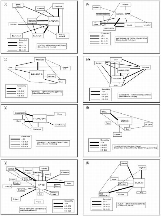
Note: a The Belgium national scale was conflated with the Brussels regional scale.

Comparing intra-regional linkages

We can take this analysis deeper by looking at individual connections within each of the eight MCRs (Figure 3.2a–h). In each, the pair of cities in the region with the largest link is designated as the prime link of the region. For comparative purposes, this link is again scored as 100 and the values of all other links are computed as proportions of the prime link. Table 3.8 presents a summary of the larger linkages.

Figure 3.2 Comparative intra-regional linkages for First Cities in each MCR

Table 3.8 Major intra-regional linkages

a Major linkages to the First City

b Major linkages that by-pass the First City

The eight prime links are shown in the first column of Table 3.8a. Each involves the First City of each region and one other major city. First Cities are identified as the city in each region with the highest global connectivity, as measured in previous GaWC research (Taylor, 2004b). It is particularly important to stress that the methodology used here analyses each region separately, so it is not possible to say that one prime link is larger than any other: they are each simply the largest in their respective regions. But it is possible to look at relative patterns of links and their sizes across regions – and it is this that makes the analyses useful in understanding comparative levels of polycentricity.

The second column of Table 3.8a shows the 11 other highest links to the First City of each MCR. This list has to be interpreted with care. Links to Paris are conspicuous, totalling four in all. What this shows is that in this MCR the prime link (Paris–Rouen) is not particularly dominant. This implies that Paris is at the centre of a region with a number of similar links, possibly indicating the primacy of Paris. South East England, Greater Dublin and Rhine-Main each have two major First City links, again implying that the prime link is not particularly dominant in their respective regions. Again, this might indicate primacy in these three regions. The other link in the table features Düsseldorf and it will be shown in the analysis below that in this case a rather different situation prevails.

Table 3.8b shows the highest 15 links that do not include the First City. There is one remarkable feature of this list: the majority, nine, of the links are from just one MCR, RhineRuhr. This is undoubtedly an indication of the polycentricity of this region. Clearly in this region not all major links are to Düsseldorf: five other RhineRuhr cities feature here. The Randstad is the only other MCR to feature prominently in Table 3.8b with three links other than to Amsterdam listed. Again this implies a degree of polycentricity. Of the other six MCRs, three (Central Belgium, Rhine-Main and South East England) have just one link each listed and three (Greater Dublin, Paris Region and EMR Northern Switzerland) are not represented at all. This further suggests primacy for the latter three and note also that the South East England link (Reading–Southampton) only qualifies for the list at the threshold level.

What can be said comparatively about the intra-regional linkages? From this evidence, three statements appear to be reasonable summaries:

• Paris Region, Rhine-Main, Greater Dublin and perhaps South East England appear to be relatively primate MCRs.
• RhineRuhr appears the most polycentric MCR, and the Randstad region also appears to be polycentric.
• It is not clear whether the Central Belgium and EMR Northern Switzerland are primate or polycentric.

Conclusion

The results reported above for North West European MCRs are unique for both Europe and the world. Business practice – office network location decisions – have been used to estimate inter-city links based on a very large sample of firms (almost 2000) for the first time for MCRs. The findings consolidate and give specificity to our understanding of the regions under study. The basic findings on service network connectivities are as follows:

1 South East England is a strongly single-node region serviced through London. With global links London dominates further but other cities, notably Reading and Cambridge, do have moderate global connections.

2 The Randstad ranks second in multi-nodality. The MCR is interconnected through two major cities, Amsterdam and Rotterdam, supplemented by the medium-level connectivity of Utrecht and The Hague. For global links Amsterdam dominates but Rotterdam remains important, with Utrecht and The Hague being moderately connected.

3 Central Belgium is largely a dual-nodality region serviced through Brussels and Antwerp. However global links are very strongly dominated by just Brussels, with Antwerp and Ghent being only moderately connected.

4 RhineRuhr is the most polycentric MCR. At the local scale Düsseldorf and Cologne dominate approximately equally but this is not a dual-nodality pattern: there are six importantly connected nodes in the region. At the global level, Düsseldorf dominates in service linkages but Cologne remains important, and Dortmund, Essen, Bonn and Duisburg drop to moderate levels of connectivity.

5 Rhine-Main is a strongly single-node region serviced through Frankfurt. This is appreciably accentuated with global links.

6 EMR Northern Switzerland is a dual-nodality region serviced through Zürich and Basel, although the latter city is relatively less important than other ‘second cities’ in duality patterns. At the global level Zürich’s connectivity dominates at the global level, but with Basel maintaining a high moderate level of service connectivity.

7 The Paris Region is a strongly single-node region serviced through Paris. With global links Paris’ dominance increases but less so than for other such regions: Rouen, Orléans and Reims all have moderate global connections.

8 Greater Dublin is a strongly single-node region serviced through Dublin. With global links Dublin overwhelmingly dominates to a remarkably extreme degree.

These results are significant in modifying the preliminary and tentative conclusions about polycentricity that we were able to reach, on the limited evidence of commuter flows, at the end of Chapter 2. But some caveats, which will emerge from the interview results in Part 3, should be noted because they prove to be of vital importance. The quantitative analysis of MCR connectivities cannot take into account the intensity or quality of actual interactions between the cities. Although RhineRuhr has the most even distribution of regional scale connectivities of the eight MCRs studied, it is only by examining actual flows and knowledge transfers that we can evaluate the strength of inter-city functional relationships and their contribution to regional polycentricity.

Further analysis is especially important because, in order to measure polycentricity quantitatively, it is necessary to calculate the regional linkages between cities for each MCR individually; thus it is not possible to compare connectivity values between the regions. Taking the example of RhineRuhr again, First City Düsseldorf is shown by GaWC global city network analysis as having the lowest overall global APS connectivity of any of the POLYNET First Cities (Taylor, 2003, Table 1). The intensity of its actual intra-regional connectivities could therefore be weaker than those of the other regions; this cannot be evaluated from the comparative analysis presented thus far. The strength of the quantitative study is that it maps potential inter-city connectivities, generated by knowledge-based APS, which cannot be revealed from analysis of official statistics. These potential connectivities, of key relevance for the ESDP (European Spatial Development Perspective) priorities to promote balanced development through cooperation between cities, must then be explored using other methods.

In Chapters 4 and 5, we go on to tackle the central but difficult task of seeking to quantify the actual flows of information between individuals and firms, for which the analysis in this chapter has provided such a vital surrogate.

Note: This Research Bulletin has been published in P Hall and K Pain (eds) (2006) The Polycentric Metropolis: Learning from Mega-City Regions in Europe London: Earthscan, pp. 53-64