GaWC Research Bulletin 192

This Research Bulletin has been published in Regional Studies, 42 (1), (2008), 1-16.

doi:10.1080/00343400601145202

Please refer to the published version when quoting the paper.

(Z)

A Global ‘Urban Roller Coaster’? Connectivity Changes in the World City Network, 2000-04

P.J. Taylor* and R. Aranya**

Abstract

A network model is used to assess the nature of change in inter-city relations from 2000 to 2004. Data are collected for 2004 on the office networks of the same global service firms that were used to describe global connectivities for 315 cities in 2000. This allows a new cross-sectional geography of connectivities to be produced for 2004, and for changes in connectivities between 2000 and 2004 to be computed. Simple visualualisation and statistical techniques are used to explore the data. A distinction is made between ‘normal change’ and ‘exceptional change’ and only two cases of the latter are definitely identified: cities in both USA and sub-Saharan Africa are generally losing global connectivity in relation to the rest of the world. Thus ‘normal change’ predominates and we conclude that contemporary inter-city change does not correspond to Castells’ image of an ‘urban roller coaster’.

Introduction: changing inter-city relations

This is an empirical paper that measures and interprets recent changes in inter-city relations at the global scale. How we understand changing inter-city relations depends on the way in which those relations are conceptualised. Traditionally, cities are arrayed hierarchically so that change is about cities ‘moving up or down’ in a zero-sum game. In the study of world cities this position is represented by FRIEDMANN’s (1986) ‘world city hierarchy’ and its subsequent updating as ‘a hierarchy of spatial articulations’ (FRIEDMANN 1995, 23). The consequence of this approach is that change derives from inter-city competition; just such a model of ‘competitive cities’ has dominated thinking generally on changing inter-city relations (LEVER AND TUROK 1999). Thus for FRIEDMANN (1995, 23) world cities

‘are driven by relentless competition, struggling to capture ever more command and control functions that comprise their very essence. Competitive angst is built into world city politics. (p. 23)

A similar Darwinian image can be found in CASTELLS (1996) use of SASSEN’s (1991) global city concept wherein change results from ‘fierce inter-city competition’ (p. 382). For FRIEDMANN the outcome is ‘inherent instability’ in a very ‘volatile’ pattern of inter-city change (p. 23, 36), for CASTELLS it is an ‘urban roller coaster’ (p. 384).

It is our view that such statements from very influential writers in the field grossly under-estimate the stability in world city inter-relations. In this paper we employ a network model of inter-city relations based on advanced producer service firms ‘inter-locking’ world cities through their worldwide distributions of offices ( TAYLOR 2001a, 2004a). The resulting world city network, like all networks (THOMPSON 2003), is ultimately sustained by mutuality among its components: contra Friedmann, in this approach the ‘essence’ of inter-city relations is co-operation. Such modelling does not, of course, mean that there is no competition between cities; we agree with BEGG (1999, 807) that ‘(p)lainly cities compete … (e)qually cities co-operate’. But in our argument, the co-operation process is prioritised because it entails the basic reproduction of the inter-city relations. Competition is less fundamental but still significant. Thus in our empirical studies of inter-city relations for 2000 we have recorded a network with hierarchical tendencies ( TAYLOR 2004a).
Of course, any empirical study of change will produce some cities doing better or worse than others. In the competitive model, such changes are interpreted as cities rising or falling in the hierarchy. Viewing cities as networks, on the other hand, leads to arguments about cities improving, consolidating or reducing their nodal location within the network. But these alternative interpretations are not in themselves useful for empirical evaluation: how do we distinguish between Friedmann’s ‘inherent instability’ and the expectation from our network model of more stability in inter-city relations? It is a matter of degree, yes, but what degree? Obviously a situation where opposite interpretations can be drawn from the same empirical evidence is unsatisfactory because it tells us about the model used, not about the changes in inter-city relations themselves. How can we ensure that our use of a network model does not predispose our empirics towards findings of inter-city stability? We confront this problem at two levels.

First, the network model can and does incorporate ‘hierarchical tendencies’ as previously noted. In this paper, we use network connectivity within the interlocking model ( TAYLOR 2001a) to measure change. This enables both ‘horizontal’ and ‘vertical’ relations to be identified (TAYLOR, CATALANO, WALKER and HOYLER 2002). There is no equivalent incorporation of anything other than competitive processes in hierarchy modelling. In addition, this specification provides the key advantage of providing quantitative measures of inter-city changes based upon large data matrices; hierarchical city studies have created no equivalent measurement or data to assess world city changes. ¹

Second, we model change in such a way as to allow notions of both ‘instability’ and ‘stability’ to be recorded. Since change is ubiquitous we interpret stability not as an outcome (‘no change’) but as a process. This process is change as myriad small forces that generate a normal distribution. Deviations from such a distribution of changes are interpreted as large forces that are distorting the normal pattern. The latter are systematic biases in change patterns that can be statistically tested and evaluated. They represent forces that are not reproducing the normal distribution and therefore can be interpreted as reflecting exceptional change in competitive processes. We think this conceptualising of stability/instability contrast as normal/exceptional change contrast to be a realistic approach to revealing or not revealing a global ‘urban roller coaster’.

This paper builds upon the first phase of interlocking modelling that produced cross-sectional measurement and analyse of the world city network for the year 2000 (TAYLOR, CATALANO and WALKER, 2002a, 2002b, 2004a; TAYLOR, CATALANO, WALKER and HOYLER 2002; DERUDDER, TAYLOR, WITLOX and CATALANO, 2003; TAYLOR, 2004a). These results were derived from a database of 100 global service firm office networks across 315 cities worldwide. In the second phase of this research, we have updated this matrix for 2004 and therefore can measure differences for 2000-04. Thus the research adds a time dimension to the cross sectional analyses for 2000. The argument is developed in five sections. First, we briefly provide a resume of the world city network model, its data requirements, and the measurement of connectivity. The second section describes the problems involved in replicating the 2000 data collection exercise for 2004, details the resulting matrices used in subsequent analyses, and specifies the way in which we measure change. Our results are presented in two ways. In the third section we provide an initial introduction to the results through some simple visualisations. These ‘tasters’ are important for getting a feel for the data, model, and results before the statistical analyses. Fourth, in the statistical analysis we identify systematic biases of change away from normal distribution expectations. In a final conclusion we interpret our findings in relation to the ‘change/stability’ debate.

The Inter-Locking Model of Inter-City Relations

This section summarises detailed description of the model and its application from earlier publications (TAYLOR 2001a; TAYLOR 2004a).The important point to make is that the measures reported below are descriptions of a process, the servicing of global capital, which is modelled as world city network formation by advanced producer service firms. This is completely different from maps of infra-structural flows (airlines, internet, etc.) that depict general network patterns (see, for instance Choi et al 2006). This study is about a specific process (stimulated by Sassen (1991/2001) and subsequently used by Castells (1996)) and is not, therefore, a general survey of how cities are faring in globalization.

To make this paper freestanding the following points need to be understood.

• The basic agents of world city network formation are global service firms with their worldwide office networks
• These firms ‘interlock’ cities into a network in the course of the practice of their work to produce the world city network
• Intra-firm flows of information, knowledge and direction can be estimated from the size and functions of pairs of city offices
• In this way relations between cities can be computed as the sum of many intra-firm estimated flows
• Aggregating for individual cities, a measure of that city’s network connectivity – the importance of its location in the network – can be derived. This is the measure employed throughout this paper and it can be specified as follows.

A universe of m advanced producer service firms located in n cities is defined. The service value of a firm j in city i is defined as the importance of its office in the city within its office network and is represented by v ij. An n x m array of all service values defines the service value matrix V.

From the service value matrix V, a basic relational element is derived as

r _{ab, j} = v _aj . v _bj (1)

This is an elemental interlock between city a and city b in terms of firm j. Aggregate city interlock can then be defined as

r_ab = ∑ r_{ab, j} (2)
          ^j

Each city could have n - 1 such links i.e. one to all the other cities in the matrix. The overall situational status of each city within the network can thus be defined as:

N_a = ∑ r_ai (where a ≠ i) (3)
          ⁱ

N a is the global network connectivity for one city a. To ease interpretation (N a will vary with size of matrix) the proportion to highest connectivity is defined as:

P_a = (N_a / N_h ) (4)

where N h is the highest network connectivity recorded in the network. This is the measure widely used in the earlier studies for 2000 and will initially be employed below. For a more detailed discussion of the interlocking network model readers are referred to Taylor (2001a; 2004a).

The data requirements for such an analysis are quite straightforward (TAYLOR CATALANO and WALKER 2002a; TAYLOR 2004a): the m firms and n cities have to be identified and service values allocated for each firm in each city. In the 2000 data collection 100 global service firms were selected ( 18 in accountancy, 15 in advertising, 23 in banking/finance, 11 in insurance, 16 in law, and 17 in management consultancy) and their office networks identified across 315 cities. Selection was based upon sector rankings of firms, number and location of offices, and availability of information on offices. Service values were derived from information on the size and functions of offices with scores ranging from 0 for no presence in a city to 5 for the firm’s headquarter city. Typical offices were scored 2, offices lacking in basic size or function were scored 1, large offices were scored 3 and offices with special important functions were scored 4. Most of the information was derived from firm’s websites, the result was vast differences in types of information available and therefore service values were allocated on a firm-by-firm basis. The end-result was a 100 firms x 315 cities array of service values, thus operationalising V, the services values matrix for which the equations above are given. For a more detailed discussion of this measurement methodology readers are referred to TAYLOR et al (2002a).

Measuring Global Network Connectivity – Phase II

Methods employed in the second phase of the world city network research were identical to those used in 2000 to enable direct comparability of the results. Though the process of data production and analysis were consistent, a brief overview is given here for the purpose of highlighting some unavoidable changes.

‘GaWC 100’ to ‘GaWC 91/ 80’ – Alterations to the Data Matrix

Since the aim of the project was to compare city connectivities in the world city network over time, it was necessary to maintain a consistency in the data structure. Thus new data collection focussed only on the original 100 firms and 315 cities. However while the latter remained constant, we were unable to exactly replicate the 100 firms.

Data gathering for the second round of analysis in 2004 was faced with a specific problem that illustrates the dynamic nature of the global economy. Of the 100 advanced producer service firms from 2000, 2 firms were liquidated completely, 5 firms had to be deleted because of mergers with other firms in the data, and 2 firms were excluded because of the low quality of data on their 2004 web pages. This resulted in a new list of 91 firms that could be used for calculating connectivity for 2004. However, even after these deletions, we were unsure of the comparability of new data with old data for 11 additional firms. Basically firm reorganization meant that information available for the two dates was quite different for these particular firms. Some of these issues were typical of accountancy firms that are often organised in membership networks: information on offices of members, which was available in the public domain in 2000, is now only accessible to clients when they are referred by a centralised contact in the networking organisation. While, the issue is most common in accountancy (6 out of the 11 firms), some advertising firms and management consultancies also no longer differentiate among their offices in terms of organisational hierarchy. Since we wish to be sure that measurement of differences between 2000 and 2004 represents economic geography change rather than data collection change, a smaller set of 80 firms is identified. It is this data set that is used in analyses below.

Table 1 gives a comparative distribution of firms across sectors for 2000 and 2004. Note that the data changes from 2000 to 2004 have affected the accountancy sector the most, with number of firms included in the data almost reduced by a half. However, because accountancy firms have much larger presence in terms of offices across the world than other services in our data, it means that, to a certain extent, the losses of connectivity due to this bias are reasonably evenly spread out, rather than having a regional pattern. With respect to other sectors, changes in the matrix may have led to increased influence of law and management consultancy in dictating network structure. However, overall we think any bias resulting from the changes is minimal.

New Calculation of Global Network Connectivity and its Change

The proportionate measure of global network connectivity (P_a in equation 4) is useful for listing cities in order of connectivity and comparing ranks, which we do below, but it has severe limitations as a way of understanding change. P_a is a closed number system that distorts the measurement of change. However much more connected it becomes, the leading city cannot show additional connectivity through its P_a connectivity measure of unity. And, of course, in ranking lists, the higher the rank the less the ability to make large leaps in rank: the city ranked 125^th can jump 20 places, the city ranked 5^th cannot. Ranking differences can have only limited utility for understanding change; below we use them just as starting point for the discussion. An additional, alternative way of measuring change is required.

Returning to the original measure of connectivity (N a in equation 3) is not a solution because the sizes of matrices have changed (there is more connectivity in the 2000 matrix because there are more firms, and anyway the large numbers with this measure are very unwieldy). Thus we standardised connectivity for both 2000 and 2004 as follows:

S_a = (N_a - N_i) / α _N (5)

where N_i = ∑ N_i / n

and α _N = √ ( ∑ (N_i - N_i )² / n)

This produces an open number sequence pivoting on zero.

Change in connectivity is first measured by:

C_a = S_{a (2004)} - S_{a (2000)} (6)

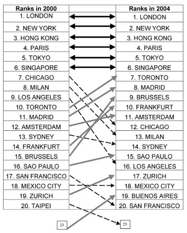
For analysis of the distribution of change, C_a is further standardised to obtain standardised change in connectivity which is defined as:

Z_a = (C_a - C_i) / α_C ) (7)

where C_i = ∑ C_i / (n-1)

and α_C = √ ( ∑ (C_i - C_i)² / n)

Results presented below will concentrate on analysis of the measures P_a, S_a , and Z_a as defined by equations (4), (5), and (7).

Change in the World City Network, 2000-04: I Visualizations

With large data sets it is important to understand the data through initial explorations of its patterns. We use elementary visualisations to this end. This approach allows us to literally see the data in various skeletal forms in order to provide some sense of the data.² This will provide suggestions for subsequent statistical analyses and aid in interpreting the statistical results.

We present the visualizations at three levels of cities. First, we look at the leading world cities and concentrate on changes in ranking for the top 20 connected cities in 2000 and 2004. Second, we follow the main analyses we previously performed on the 2000 data and identify a roster of significant cities with P_a values of at least 0.2 (in practice one fifth of London’s connectivity). A new cartogram showing the worldwide pattern of change is presented. Third, this geographical distribution of significant cities change is followed by discussion of the statistical distribution of all 315 cities as portrayed in a change histogram. In this section we elaborate on the normal distribution process and begin the task of searching out systematic biases, winners and losers beyond the normal distribution of change. As such this section acts as the link between visualizations and the statistical analyses.

Change in Ranks among Top 20 Cities

The easiest method of showing change is to use city ranks in 2000 and 2004. Just such a comparison is illustrated in Figure 1 to provide a visualisation of the changes in the top 20 world cities. Cities have been ranked according to their global network connectivity in the world city network, as represented by the 315 cities used in the study.

The visualisation gives a very clear picture of change in the top echelons of the world city network. Noteworthy aspects are:

• There is stability in the top 6 ranks showing that the world city network is constant as far as the ‘big six’ cities are concerned – London, New York, Hong Kong, Paris, Tokyo and Singapore have retained their dominance of the network. In addition they have retained their positions with respect to each other indicating constancy in the complex roles they perform in the network.
• Considerable shuffling of cities has taken place below the ranks of the ‘big six’. The most significant losers are – Chicago, Milan, Los Angeles, Sydney, San Franciscoand Taipei. The big gainers are – Toronto, Madrid, Frankfurt, Brussels, Zurichand Buenos Aires.
• The patterns that are most obvious in the changes in ranks are – loss in position of large U.S. cities with the exception of New York, rise of important European capital cities such as Madrid and Brussels, and the increasing importance of Toronto as compared to other North American cities. The veracity of such patterns of change is assessed further for all 315 cities below.
• Despite these changes there is only two entries/exits to/from the top 20: the inclusion of Kuala Lumpur and Buenos Aires and the exclusion of San Francisco and Taipei. The rise of Buenos Aires might seem unexpected given the financial collapse of the Argentine economy in 2001, but it should be noted that economic difficulties provide an increased market for some producer services.

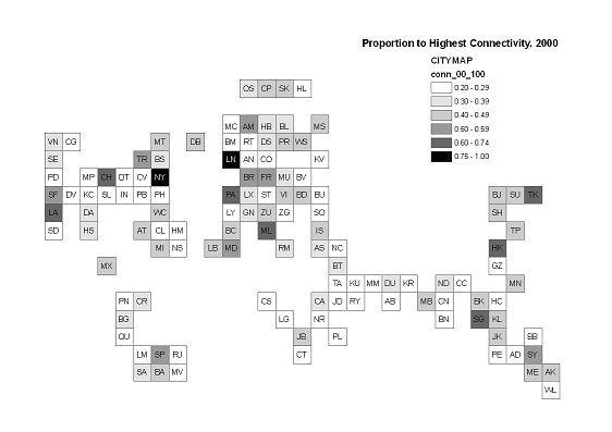
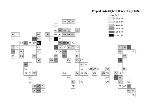
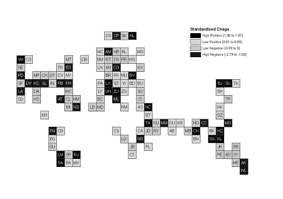
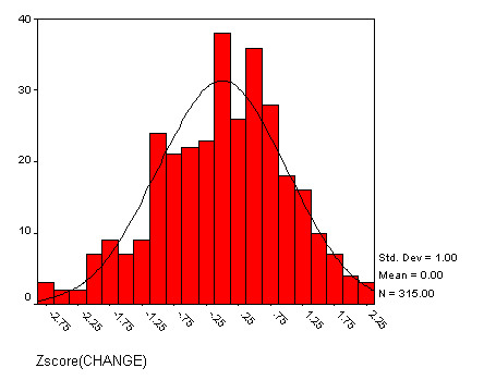
Clearly Figure 1 displays a mixture of stability and change among the leading cities of the world city network; we conclude tentatively that stability appears the more dominant feature of connectivity among leading world cities. This is an interesting and suggestive starting point – a visual taster of things to come - but it does not begin to do full justice to the data we have collected. As an ordinal measure it loses information provided by the actual connectivity measures but, more important, the figure does not tell us anything below this limited number of leading cities. Here we reach the Achilles heal of simple visualisation: it cannot accommodate large numbers of changes into a single diagram. But a critical feature of our interlocking model approach has always been its incorporation of relatively large numbers of ‘cities in globalization’ rather than just a few select world or global cities (TAYLOR 2004a, 42).

New Connectivity Cartograms of Significant Cities

In the 2000 analyses ( TAYLOR 2004a), the findings for connectivity were presented for the 123 cities with the highest connectivities (as previously mentioned, the cut-off point for inclusion being cities with at least one fifth of London’s connectivity). This number of cities provided a suitable quantity for depiction on a simple cartogram ( TAYLOR 2004a, 71-2). The resulting diagram of connectivities (using P a from equation 4 above) shows the geography of significant cities in the world city network for 2000 ( TAYLOR 2004a, 73). This cartogram is reproduced here as Figure 2 for comparative purposes.

Replicating this methodology for 2004 data produces the geography of significant cities in the world city network for 2004 (Figure 3). The first point to make about this new diagram is that the roster of cities is different. In 2004 there are only 107 cities in the roster (i.e. with P_a above 0.2), a net loss of 17. The exit/entry cities are listed inTable 2 . The first column shows the cities dropping out to be largely less important US and European cities plus minor financial centres (Hamilton, Panama City, Manama and Nassau); of those outside these categories the exclusions of Nairobi and Lagos are the most interesting in that it leaves inter-tropical Africa with no ‘significant’ city in 2004 (note another African city, Casablanca, also drops out). The second column shows the newly ‘significant’ cities for 2004, the key features here is the inclusion of four central American capital cities and two UK cities; outside these categories the inclusion of Osaka is the most interesting in that this ‘second city’ (HILL and FUJITA 1995) of the world’s second largest ‘national economy’ was a surprise omission from the 2000 roster. But these alterations to the shape of the cartogram are only the marginal changes around an arbitrary cut-off level; the prime interest is in comparing the geographies of connectivity in 2000 (Figure 2) and 2004 (Figure 3). The diagrams use a quite detailed division of city connectivities (6 levels are mapped) and yet we find very similar geographies. In all regions, apart from changes reported in Table 2, geographies are very similar: it is the same cities with highest connectivities in every part of the world. In conclusion, this comparison of the two cross-sections suggests stability in the geography of connectivities.

Acceptance of this finding requires support from actual change measures. In Figure 4, changes in connectivity for the 123 significant cities in 2000 using 2004 data are shown for Z a (equation 7). The first point to make about this map is that there is a very mixed geographical distribution of positive and negative changes. This supports the stability conclusion above. But there are suggestions of systematic geographical biases in change. The most obvious is in the USA where negative change clearly dominates positive change; this contrasts with Europe where the changes appear to be much more balanced. However, to fully explore systematic patterns in connectivity change we need to consider all 315 cities.

The Statistical Distribution of Connectivity Change

Depictions of comparison and change among selected major cities provide many hints about the nature of variation in the world city network between 2000 and 2004 but full assessment requires use all 315 cities in the data sets. Thus we concentrate on 315 connectivity changes (Z_a in equation 7): the prime advantage of such a large number of changes is that we can explore the statistical distribution: frequencies of city changes are depicted in Figure 5 where the histogram is compared to a normal distribution. Before this comparison is described we need to indicate the importance of the normal distribution.

Cities and their inter-relations are very complex phenomena and there are infinite influences and forces that are forever changing them. In such a situation where myriad small forces are contributing to change, both reinforcing and counteracting each other in endlessly intricate ways, the expected pattern of change measures is a normal statistical distribution. On the other hand if there are any large systematic forces influencing change, this will be reflected in deviations from the normal curve. Here we look for such deviations as a prelude to statistical testing for systematic forces. Thus we will treat marked differences from normal as indicating possible major influences distorting the myriad small forces process. Through investigation of the distribution we will identify cities associated with ‘non-normal’ change that will suggest (with previous discussions above) hypotheses to test in the next section.

Because we use standardised measures in Figure 5, the mean is zero and the standard deviation is unity but skewness and kurtosis can vary. These are computed as skewness = -0.298 indicating a modal bias towards negative changes (compared to normal) and kurtosis as –0.165 indicating leptokurtosis, a bias towards a flat centre and enlarged tails. However, neither measure is particularly instructive because the centre of the distribution is bimodal. This latter feature is, in fact, a gross departure from normal and does indicate that the myriad small forces model is appreciably distorted (i.e. there are large forces to be identified).

Visual inspection of the distribution (Figure 5) suggests the following elements.

• The bimodal centre indicating fewer than expected zero (or near-zero) changes
• A three step negative profile starting with an enhanced tail and progressing to separate ‘rectangular’ sections
• A smooth and quite normal profile of positive change but culminating in a deficiency at the tail.

We can interpret the first two patterns as indicating more or less cities indicating particular important forces affecting negative change. In contrast the third pattern suggests that positive change has not been the result of any particular forces.³ We go back to the original ranked list of 315 changes to select cities representing the patterns described above. Basically we list the sizes of the 314 differences between ranked cities and identify the large gaps to indicate possible changes in process.

Using this method we compile four lists of cities: the ‘hole’ in the middle of the distribution, the ‘third mode’ in the negative profile, and for comparison, the two tails. The first two lists of cities are shown in Table 3. The dearth of low positive change (the ‘hole’) is represented by the list in the first column. Since this is an example of where ‘missing’ cities are not found (and they cannot be known), the cities that are found here should not exhibit any particular pattern. And this is the case – it would be hard to imagine a more motley collection of cities! In contrast we can search for a pattern in the second column which represents an excess of medium negative change. Of course, we cannot know which are the ‘additional cities’ in the list above and beyond what would be normal, but the fact that a third of these cities are US cities (9 out of 27) does suggest a strong process operating to the detriment of US connectivity changes, something previously noted.

Lists of cities in the two tails are shown in Table 4. We have chosen large gaps in the change ranks to find approximately 25 of the most negative and positive change cities. The first thing to note is that in comparing lists the negative changes are larger than the positive changes through all ranks (e.g. the largest positive change ( Edinburgh’s 2.301) is a smaller absolute value than 5 th largest negative change ( Nairobi’s –2.390)). In addition, all large gaps between ranked cities (> 0.04) are indicated and the negative tail list has more of these (12 compared to 9) and they are generally larger. This indicates a more ‘bumpy’ negative tail and is consistent with our previous recognition of a smoother positive profile through visual inspection of Figure 5. In terms of patterns of cities the US effect can be seen again: there are 5 US cities in the negative tail but none in the positive tail. Otherwise other patterns are hard to discern in the negative tail: two New Zealand cities and two minor financial centres are the only pairs of ‘like-cities’. Of course, the myriad small forces model produces ‘random’ cities in the tails of normal distributions and Figure 5 shows little excess of cities in the negative. In the positive tail, Figure 5 actually shows a dearth of cities so we expect no patterns here. We do, however, have one suggestion – capital cities seem to be well represented: 13 out of the 24 cities are state capitals. (Although not state capitals, Edinburgh and Cardiff as newly devolved UK ‘national’ capitals do suggest the same advantage for ‘political cities’). Otherwise, there are only the odd specific suggestions for the high positive change such as Sarajevo and Belgrade recovering from the 1990s Balkan wars and Bratislava becoming the capital of a new state.

We have taken visual inspection of change results about as far as we can. The next step is to convert some of these ideas for statistical testing.

Change in the World City Network, 2000-04: II Statistical Analyses

Descriptions of changes in rank, geographies of connectivity, and distributions of connectivity changes have raised a number of hypotheses about the inherent structure, if any, in the dynamics of the network of cities being studied here. For example, results from various comparisons indicate loss of connectivity among American cities or, in the last section, a tendency for positive change among capital cities. These and other suggestions are combined with recent literature that provides hints for change to create hypotheses for testing. Significant results from the latter are then fed into a multiple regression analysis to model changes in connectivity and show how important the systematic distortions are individually and collectively.

Statistical Testing of Systematic Factors Producing Connectivity Change

Three sets of hypotheses are tested:

1. There is a simple political hypothesis focusing on state capital cities. The question we ask is: are capital cities more likely to experience positive change in connectivity? Here we are searching for a systematic political force influencing changing positions of cities in the world city network as suggested above. World cities are typically important political cities ( TAYLOR 2005a, 2005b). Capital-city functions are common in world cities and although there are no political variables in our definition of the world city network, states are important markets for advanced producer services (ELMHORN 2001). Thus capital cities are attractive locations for major service offices. The reason why we suggest this force may be changing between 2000 and 2004 is that the world-economy was less buoyant in the first years of the twenty first century compared to the final years of the twentieth century and it may be that states have been picking up the slack in the market enabling globalization to continue apace.
2. There are two concentration/dispersion hypotheses that relate to SASSEN’s (1994) emphasis on the simultaneous concentration and dispersion of activities in economic globalization.
1. Has there been a concentration of additional connectivity in the ‘global cities’? We interpret the latter as the top 25 cities as defined in the 2000 connectivity analyses ( TAYLOR 2004a, 99). If indeed global cities are a ‘new type of city’ unique to contemporary globalization as SASSEN (2001, 4) insists, then we can suggest that they should be especially prospering with continuing globalization of the world-economy. There were initial hints at this in an earlier study of change (TAYLOR, CATALANO and GANE 2003).
2. Are thesecondary cities within countries emerging from the ‘shadow’ of the prime city in each country? In other words, as globalization proceeds, is it extending beyond the main city in a country to ‘second’ other cities previously relatively neglected? For instance, BEAVERSTOCK et al (2000a) have suggested a ‘ New York shadow effect’ on other US cities. However, the classic ‘second city’ case is usually taken to be Osaka and its ‘ Tokyo problem’ (HILL and FUJITA 1995) and we noted above how this city has become appreciably more connected. More generally, recent literature from several countries has suggested cities beyond the main city in a country have been ‘catching up’ (AGUILAR 1999; IPEA et al 2001a; GEYER 2003; LANG 2003; PARKINSON et al 2004; ROSSI and TAYLOR 2006). The researches reported in these publications each deal with a particular country; here we investigate whether this is a more general process.
3. We have generated global geographical hypotheses. In FRIEDMANN’s (1986, 1995) hierarchical allocations, cities in the semi-periphery are explicitly included suggesting an important diffusion across the world-economy. This position has been further developed by SASSEN’s (2000, 151), who asserts that there is a ‘new geography of strategic places’ that ‘cuts across … the old North-South divide’.
1. (a) Thus we begin with original North-South divide as depicted by the Brandt Report (INDEPENDENT COMMISSION ON INTERNATIONAL DEVELOPMENT ISSUES 1980). Are cities in the ‘South’ relatively enhancing their city connectivities?
2. (b) But this ‘South’ is a quarter of a century old and much has happened since then, including, of course, the globalization processes that are our subject. Thus we define a ‘new South’ defining ‘less developed’ regions as found in 2005 – Pacific Asia is omitted (see Taylor et al 2006) and ex-USSR countries beyond the Black Sea are added (new republics in Caucasian Europe and Central Asia – see UNDP (2004)). Are cities in the ‘new South’ relatively enhancing their city connectivities?
4. We have generated regional geographical hypotheses: rather than reforming the ‘South’ as a category it is argued that whatever unity the ‘South’ category had, it has now splintered into different regions with different reactions to globalization. The general hypotheses is: are there differences in patterns of change based on cities in selected world regions? This relates to the basic finding in cross-sectional studies using the GaWC 100 data that globalization through advanced producer service activity is largely regional in pattern (TAYLOR et al 2002b, 2004; TAYLOR 2004a, 2004b; DERRUDDER et al 2003). This relates to globalization as an ongoing set of processes that are having different outcomes over time and place. Many of the processes reflected in the data used here have involved economic practices developed in the world-economy core (for instance management consultancy in the USA) and which have subsequently expanded into other regions at different levels of penetration. We select important world regions that have been shown to be distinctive in studies of the data for 2000 ( TAYLOR 2004b), 4 from the core zone and 4 from non-core zones.
1. United States cities. We know from the 2000 cross-sectional analyses that these cities are less globally connected than their European peers (LANG AND TAYLOR 2004), from evidence above it would seem that negative changes are increasing this feature.
2. Western Europe cities. The inverse of the above: have these cities become more globally connected ( TAYLOR and DERUDDER 2005)?
3. Pacific Asia cities. This region has been the globalization success story: is global integration of its cities continuing apace (TAYLOR et al 2001)?
4. East European cities . We define this category as ex-COMECON countries east of the Black Sea whose cities have integrated immensely since 1990: is this process continuing ( TAYLOR and DERUDDER 2005)?
5. Sub-Saharan Africa cities. The poorest region in the world, evidence above suggests reduced connectivities and this was also found in initial analyses of change (TAYLOR, GANE and CATALANO 2003).
6. ‘Greater’ Middle East cities. This region extends from Mediterranean Africa to Central Asia, traditionally a city-rich world region, its cities appear not to have prospered with globalization ( TAYLOR 2001c): there are indications from above that its city connectivities are beginning to catch up.
7. Latin America cities . Indications from above, especially for Central American cities, suggest increased city connectivities for this region.
8. South Asia cities . India appears to be following China’s lead in globalised economic growth: is it reflected in enhanced city connectivies?

Each hypothesis is statistically assessed using the simple binomial test (SIEGEL 1956, 36-42). For every hypothesis there is a set (sample) of n cities. These are divided into those that show negative change and those that show positive change. The test focuses on the smaller of these two frequencies, s. It is known that where the negative and positive changes for a population are the same, the following expression approximates a normal distribution (p. 41):

z = ((s ± 0.5) – (n x 0.5)) / √(n x 0.25)     (8)

so that the probability of z occurring in a sample by chance can be found.⁴ This probability is used to test imbalances between positive and negative change using the conventional level of 0.05 as the cut-off level for defining a statistically significant difference.

The results of applying this test are shown in Table 5. The table shows the frequencies of cities recording negative and positive connectivity change: these columns emphasize that our hypotheses are about tendencies not absolutes: there is no category with all positive or all negative change. However, of the 13 hypotheses, 7 have probabilities that indicate a significant difference in the balance between negative and positive change:

• Capital cities are more likely to experience positive change than negative change
• United States cities are more likely to experience negative change than positive change
• Western Europe cities are more likely to experience positive change than negative change
• Pacific Asia cities are more likely to experience positive change than negative change
• Sub-Saharan cities are more likely to experience negative change than positive change
• ‘Greater’ Middle East cities are more likely to experience positive change than negative change

Note that all but one of the successful hypotheses is a regional sample of cities, confirming the basic regional structure (TAYLOR 2004b) of the world city network; these analyses extend the network structure into patterns of change. All four core regions record significant tendencies with US cities contrasting with cities from the other regions though their overall negative change. Two of four non-core regions record significant tendencies but in different directions: Sub-Saharan Africa cities are generally losing connectivity; Middle East cities are gaining it. In addition, our political hypothesis is confirmed: capital cities are more likely to experience positive change. All this means is that as well as the two other non-core regional hypotheses falling, both the global geographical and concentration/dispersion hypotheses are not supported by our analyses, indicating that Sassen’s suggestion of a lessening of the ‘North-South divide’ through inter-city relations cannot be sustained.

The above analyses provide very basic, and simple, findings in our search for systematic forces operating to influence changing city connectivities. Of the 7 significant tendencies identified, 5 are for positive changes. This is counter to our expectations from visual inspection of the histogram (Figure 5) above from which we predicted the negative slope would be where the systematic influences were more likely to be found. This contradiction is resolved in our final, more sophisticated, analysis.

A Multivariate Model of City Connectivity Change

The binomial statistical tests are a series of bi-variate analyses: they involve treating explanatory (independent) variables, the city categories, as separate influences on city connectivity change. Furthermore, by using a positive/negative dichotomy to represent the latter, a vast proportion of the variability in the dependent variable is simple not taken into account (i.e., for instance, negative values of -0.01 and –2.01 are treated as equivalent in the binomial testing). A multivariate regression analysis using 315 standardized change values (Z_a in equation 7) as dependent variable overcomes both problems. However, we do make direct use of the binomial test results: we employ just the seven independent variables from the hypotheses with statistically significant results. Thus our regression model is specified as

Z_a = f(x 1 , x 2, x 3, x 4, x 5, x 6, x 7) (9)

where all independent variables are binary measures: x₁ is capital city = 1, all other cities = 0; x₂ is US cities = 1, all other cities = 0; x₃ is Western Europe cities = 1, all other cities = 0; x₄ is Pacific Asia cities = 1, all other cities = 0; x₅ is Eastern Europe cities = 1, all other cities = 0; x₆ is sub-Saharan Africa cities = 1, all other cities = 0; x₇ is ‘greater’ Middle East cities = 1, all other cities = 0. The results of calibrating this equation as a linear model are shown in Table 6 .

The first point to make about this model is that it confirms the general binomial finding that there are systematic forces operating on city connectivity changes: the regression is statistically significant at a very low probability level. However, the relationship itself is relative weak; the correlation of under 0.3 translates into only 6% (after adjustment) of city connectivity changes being accounted for (‘explained’) by the independent variables. The corollary is that 94% of changes remain unaccounted for. This latter can be interpreted as the myriad small forces of the normal distribution process (non-systematic change or ‘stability’) that dominate Figure 5. Thus the first finding from the regression model is that changes in city connectivities between 2000 and 2004 are very largely small, non-systematic variations indicating a structural stability but that larger systematic forces are also at work, albeit to minor effect.

These systematic forces can be assessed using the regression coefficients of the independent variables (B in Table 6). These coefficients are gradients of change; they measure the change in the dependent variable that occurs with a one-unit change in an independent variable. For binary independent variables, regression coefficients are particularly easy to interpret. For example, in Table 6 the coefficient of –0.1161 for US cities means that being a US city reduces standardised connectivity by 0.1161. The first point to note about these coefficients is that despite selection from significant binomial results, not all independent variables have significant coefficients. Both capital cities and Pacific Asian cities have coefficients that are effectively zero – whether a city is a capital city or a Pacific Asian city adds or subtracts little or no city connectivity change. Thus the possibilities of these results happening by chance are high as represented by their high probabilities. These clear non-significant results differ from the binomial findings, why? There are two ways this can happen. First, changing the measurement scale of the dependent variable from binary (positive/negative) to a much more precise ratio scale will cause different results – both capital and Pacific Asian cities have cities towards the middle of the distribution where change of measurement scale will have a large effect. Second, the regression model is a multivariate technique that considers all variables simultaneously. This means that they correct bi-variate significant findings that are caused by the effect of another variable. For instance, in our analyses, the capital cities variable is inversely related to the US cities variable because only one of the latter’s 44 cities is a national capital (the bi-variate correlation r₁₂ = –0.31, the highest absolute simple correlation in our analyses). With 43 US cities automatically removed from the capital city sample, their tendency towards negative change helps capital cities to record a tendency towards positive change. In the multiple regression model, this co-linearity effect is removed and capital cities lose their statistical significance.

There are another three variables that do not record significant regression coefficients but their probabilities are low enough to suggest a possible systematic effect. Least likely are Middle East cities with a probability of nearly one in five of occurring by chance, and Western Europe cities fare only slightly better as a systematic effect. East Europe cities are a different case, not quite significant, at a one in eight chance the result is clearly suggestive of a specific regional force in city connectivity changes. But there are two regional sets of cities that do meet the significance threshold: US cities and sub-Saharan cities. Here there is strong evidence that regional forces are, in both cases, creating a strong propensity for relative loss of connectivity between 2000 and 2004: as reported above, being a US city reduces global connectivity change by about 0.12, being a sub-Saharan African city reduces connectivity change by 0.09. These two results are intriguing because the two regions represent opposite ends of the globalization spectrum, one has been the powerhouse behind global processes, the other has been the region most ‘out of the global loop’. The latter position of sub-Saharan Africa means that the relative decline of its city’s connectivity is not surprising: it has previously been shown that withdrawal from these city ‘outposts’ of global service provision has been a result of a less buoyant world-economy (TAYLOR, GANE and CATALANO 2003). The US cities result may therefore appear to be the more surprising but this is not the case: as previously reported, the global connectivities of US cities has not been what might be expected of the largest national economy in the world (TAYLOR and LANG 2004). This latter example will be considered further below in our final interpretation of results.

The key general point to be derived from the regression model is that the two significant results are for hypothesized negative changes of city connectivities. These patterns are so distinctive that their inclusion in the multivariate analysis eliminates all previous significant positive change results (due to co-linearity with cities in four regions as well as capital cities). This is consistent with the interpretation of the frequency distribution of connectivity changes (Figure 5) where we noted the uneven negative profile as a probable source of systematic changes. Thus, in this further analysis we have overturned and completely reversed the majority of significant positive change variables resulting from the binomial testing.

Summary of the Quantitative Results

Political hypothesis . There is some evidence for capital cities having significantly more positive change (binomial test) but this finding does not survive multivariate scrutiny: it is likely a co-linearity effect of US cities.

Concentration/dispersal hypotheses . There is no evidence that changes in city connectivities are related to these processes.

Global geographical hypotheses . There is no evidence that changes in city connectivities are related to these processes.

Regional geographical hypotheses . These eight hypotheses provide a range of findings. First, there is no evidence at all for systematic forces making Latin America cities or South Asia cities distinctive in their connectivity changes. Second, there are cities from 4 regions – Western Europe, Pacific Asia, East Europe and ‘greater’ Middle East - that are found to have significant results suggesting additional positive changes in the binomial test but these findings do not carry over into the multivariate model. This leaves two clear instances of systematic forces creating relative negative connectivity changes: cities in the USA and cities in sub-Saharan Africa.

Although two systematic forces have been identified, the final outcome of this statistical analysis is that well over 90% of the variation in city connectivity changes cannot be accounted for in this manner. Thus we deduce that the normal process of myriad small changes overwhelmingly dominates the way the connectivities of cities have changed between 2000 and 2004.

Conclusion

This has been a straightforward empirical paper in which we have assessed the weakly-evidenced claims of Friedmann and Castells that inter-city relations at the global scale are very unstable. Using a conceptually-sound and empirically-rich approach, we have not found evidence to support their image of an extremely competitive world of cities. Our initial focus on visualisation suggested normal stability overall, this was initially challenged by the first detailed statistical analysis, but the final statistical modelling showed systematic bias in city connectivity changes in just two regions thus moving us back to the overall conclusion supporting the normal stability process. There was no global ‘urban roller coaster’ between 2000 and 2004.

There are three considerations that should be taken into account when discussing this finding. First, there is the question of the specifics of the analyses. We have used a particular approach to understanding changes in inter-city relations that follows Sassen’s emphasis on advanced producer services and derives city connectivities from the office networks of global service firms.⁵ At the time of writing this appears to be the only large-scale method available to assess the stability of worldwide inter-city business relations.⁶ Other, as yet unknown, methods might produce alternative findings. However this would not negate our analysis but it would require modification of our interpretation. Instead of dismissing the global urban roller coaster, we would have to begin exploring the question of under what conditions this phenomenon were to be found. The challenge to those researchers who hold the extreme city competition position is to empirically turn the debate in this direction.

Second, there is one specific finding that can be used to make another important point: the relative decline of US cities in our world city connectivity analyses. It must be emphasized that our approach is a one-scale method; we have studied connectivities generated by service firms operating on a global scale. This is just one process within the service sector that is itself just one part of wider economic processes. Thus relative reduction in global network connectivity in our analysis should not be translated simply into general economic decline of a city. The US cities illustrate this situation perfectly. As profit-maximising entities, US producer service firms can choose to concentrate their investment in servicing the richest national service markets in the world and with which they are familiar, instead of chasing new clients in unfamiliar lesser markets that constitute the remainder of the world-economy. Thus it can make sense not to ‘go global’ or expand globally in order to be economically successful; in the case of law this is clearly the case (BEAVERSTOCK et al 2000b). Hence, our analyses do not indicate economic decline of US cities (TAYLOR and LANG 2005). The US situation illustrates this argument perfectly. The key point is that large US producer service firms are in a different market location to firms from other countries. As profit-maximising entities, these large US service firms can choose to concentrate their investment in servicing the richest national service markets in the world and with which they are familiar, or they can choose to compete for new clients in unfamiliar smaller markets that constitute the remainder of the world-economy. For many it will make economic sense not to ‘go global’ but to continue to thrive in the rich domestic market:; in the case of law this is clearly often the case (BEAVERSTOCK et al 2000b). Hence, our analyses do not indicate economic decline of US cities, they are highly successful producer service centres but with less of their major firms engaging in global servicing (TAYLOR and LANG 2005). New York is the exception to this tendency and this is reflected in its bucking the US trend. However, this argument certainly does not extend to sub-Saharan cities: in all probability, our analyses do provide evidence of general economic decline.

Third, there is the question of timing. If world city network change were something as dramatic as a ‘global roller coaster’, then data covering just five years would be enough to reveal it. However, more generally we can note that this is a quite short period to measure any global social change. Obviously the shorter the period the more likely findings are going to show stability. In this case we are contrasting two cross-sections generated in different economic contexts: the geographical outcome in 2000 of decisions made in the late twentieth century economic expansion against the outcome in 2004 resulting from decisions made in the more uncertain years of the early twenty first century (after the dot.com bust, Enron scandal, and collapse of the Argentinean economy). Given the dearth of other measurement of trans-state social change in globalization we have no way of knowing whether our results can be generalised beyond the four years we have studied. This paper is just a modest beginning to the task of monitoring changing relations between cities in a globalising world economy. Globalization is not itself an end-condition, it is an ongoing process (TAYLOR 2000). Our results should only be interpreted in this spirit.

REFERENCES

AGUILAR, A. G. (1999), Mexico City growth and regional dispersal: the expansion of largest cities and new spatial forms. Habitat International 23, pp. 391-412.

BEAVERSTOCK , J V, SMITH, R.G. and TAYLOR, P J (2000b) "World city network: a new metageography?" Annals, Association of American Geographers, 90, 123-34

BEAVERSTOCK J V, SMITH R G and TAYLOR, P J (2000a) Geographies of globalization: US law firms in world cities, Urban Geography, 21, 95-120

BEGG, I. (1999) Urban Competitiveness: Policies for Dynamic Cities, Bristol : Policy Press

BRUNDTLAND, G.H. (1987) World Commission on Environment and Development, Our Common Future, Oxford: Oxford University Press

CASTELLS, M (1996) The Rise of Network Society . Oxford: Blackwell

CHOI, J. H., BARNETT, G. A. and CHON, B-S (2006) Comparing world city networks: a network analysis of Internet backbone and air transport intercity linkages, Global networks, 6, pp. 81-99.

DERUDDER, B. and TAYLOR, P.J. (2005) The cliquishness of world cities, Global Networks, 5(1), pp. 69–89.

DERUDDER, B. and WITLOX, F. (2005a) On the use of inadequate airline data in mappings of a global urban system. Journal of Air Transport Management. 11 (4), pp. 231-237.

DERUDDER, B. and WITLOX, F. (2005b) An appraisal of the use of airline data in assessing the world city network: A research note on data. Urban Studies. 42 (13), .

DERUDDER, B., TAYLOR, P.J., WITLOX, F. and CATALANO, G. (2003) Hierarchical tendencies and regional patterns in the world city network: a global urban analysis of 234 cities, Regional Studies, 37(9), pp.875-886.

ELMHORN, C (2001) Brussels: a Reflexive World City. Stockholm: Almqvist and Wiksell International

FRIEDMANN, J (1986) The world city hypothesis, Development and Change 17, pp 69-83

FRIEDMANN, J. (1995), Where we stand: a decade of world city research. In P. L. KNOX & P. J. TAYLOR, eds., World Cities in a World-System. Cambridge: Cambridge University Press.

GEYER, H. S., ed., (2002), International Handbook of Urban Systems. Cheltenham, UK: Edward Elgar

HALL, P (1966) The World Cities, London: Heinnemann

HILL, R. C. and FUJITA, K. (1995), Osaka’s Tokyo problem, International Journal of Urban and Regional Research 19, pp. 181-91

INDEPENDENT COMMISSION ON INTERNATIONAL DEVELOPMENT ISSUES (1980) North-South: a Programme for Survival. London: Pan

IPEA, IBGE and UNICAMP (2001), Caracterização e tendências da rede urbana do Brasil. Brasilia: IPEA ET AL, V. 1-6.

LANG, R. E. (2003), Edgeless Cities – Exploring the Elusive Metropolis. Washington: Brookings Institution Press

LEVER, W.F. and TUROK, I., (1999) Competitive Cities: Introduction to the Review, Urban Studies, Vol. 36, Nos 5-6, 791-793

PARKINSON, M., HUTCHINS, M., SIMMIE, J., CLARK, G. and HERDONK H. (2004), Competitive European cities: where do the Core Cities stand? London: ODPM.

ROBINSON, J (2002) ‘Global and world cities: a view from off the map’, International Journal of Urban and Regional Research, 26, 531-54.

ROBINSON, J (2005) ‘Urban geography: world cities, or a world of cities’, Progress in Human Geography, 29, 757-65.

ROSSI, E. C. AND TAYLOR P. J. (2006) Brazilian Cities within Domestic and Global Banking Circles, Tijdschrift voor Economische en Sociale Geografie, 97,

SASSEN, S (1991/2001) The Global City, Princeton, NJ: Princeton University Press

SASSEN, S (1994) Cities in a world economy. Thousand Oaks, Calif.: Pine Forge/Sage.

SIEGEL, S (1956) Nonparametric Statistics for the Behavioral Sciences. New York: McGraw-Hill

TAYLOR, P.J. (2000) Izations of the world: Americanization, modernization anf globalization, in C Hay and D Marsh (eds) Dymystifying globalization, London: Macmillan

TAYLOR , P.J. (2001a) Specification of the world city network, Geographical Analysis, 33(2), pp.181-194.

TAYLOR , P.J. (2001b) Visualising a new metageography: explorations in world-city space, in G DIJKINK and H KNIPPENBERG (eds) The Territorial Factor. Amsterdam: Vossiuspers UvA 113-28

TAYLOR , P.J. (2001c) West Asian/North African cities in the world city network: a global analysis of dependence, integration and autonomy, The Arab World Geographer 4, 146-59

TAYLOR , P.J. (2004a). World City Network. A Global Urban Analysis, London and New York: Routlegde.

TAYLOR , P.J. (2004b) Regionality in the World City Network, International Social Science Journal, 56 (181), pp361-372.

TAYLOR , P.J. (2005a) Leading world cities: empirical evaluations of urban nodes in multiple networks, Urban Studies 42, 1593-1608

TAYLOR , P.J. (2005b) New political geographies: global civil society and global governance through world city networks, Political Geography 24, 703-30

TAYLOR , P.J., CATALANO, G. and WALKER, D.R.F. (2002a) Measurement of the world city network, Urban Studies, Vol. 39, 2367-2376.

TAYLOR , P.J., CATALANO, G. AND WALKER, D.R.F. (2002b) Exploratory analysis of the world city network, Urban Studies, Vol. 39, 2377-2394.

TAYLOR, P. J., DERUDDER, B., GARCIA, C. G. and WITLOX, F. (2006), From north-south to global south: a geohistorical investigation using airline routes and travel, 1970-2005, GaWC Research Bulletin No 209.

TAYLOR , P.J., DOEL, M.A., HOYLER, M. WALKER, D.R.F. and BEAVERSTOCK, J.V. (2001) World cities in the Pacific Rim: a new global test of regional coherence, Singapore Journal of Tropical Geography, 21 (3) pp 233-245

TAYLOR, P J , GANE, N AND CATALANO, G (2003) A geography of global change, 2000-2001, Urban Geography 24, 431-41

TAYLOR, P J and LANG R (2004) US Cities in the World City Network - Survey Series, Washington, DC: The Brookings Institution

TAYLOR , P.J., WALKER, D.R.F., CATALANO, G. and HOYLER, M. (2002) Diversity and power in the world city network, Cities, 19(4), pp 231-241.

THOMPSON, G.F. (2003) Between Hierarchies and Markets, Oxford: Oxford University Press

UNDP (2004) Forging a Global South: UN Day for South-South Cooperation. New York: United Nations Development Programme

Figure 1: Change in Ranks 2000-04

Figure 2:Cartogram of Connectivity for GaWC 100, 2000

Figure 3: Cartogram of Connectivity for GaWC 91, 2004

Figure 4: Cartogram of Standardised Change for 123 cities (based on GaWC 80 for 2004)

Figure 5:Distribution of Standardised Change

Table 1: Comparative distribution of firms across sectors in 2000 and 2004 data

Table 2: Changes between 2000 and 2004 for the Roster of ‘Significant’ Cities (P_a > 0.2)

Table 3: Selected City Lists Illustrating Particular Features of Figure 5

* gap between Omaha and Bogota = 0.060
gap between Yerevan and Strasbourg = 0.047

** gap between Rabat and San Francisco = 0.056
gap between Dortmund and Bonn = 0.088

Table 4: Lists of Cities in the Two Tails of Figure 5

* gap between Harare and Panama City = 0.082

** gap between Macau and Zurich = 0.056

*** all changes underlined are large gaps (> 0.04)

Table 5: Binomial tests

Table 6: Multiple Regression Model

NOTES

*Peter J Taylor, Department of Geography, Loughborough University, Loughborough , LE11 3TU, UK, p.j.taylor@lboro.ac.uk

**Rolee Aranya, Department of Urban Design and Planning, University of Science and Technology, Trindheim , NORWAY, rolee_aranya@yahoo.com

1. The empirical basis of Friedmann’s competition findings is ‘thumbnail sketches’… drawn from newspaper accounts and sporadic readings’ of the prospects of 17 individual cities .

2. For a discussion of visualization relating to earlier work on the world city network see TAYLOR (2001a and b)

3. It should be noted that we have used different scales and produced approximately the same shaped histogram: the three features above are most certainly not the product of choice categories in which to count frequencies.

4. Where n < 25 a slightly different formula is used but the process is otherwise the same (SIEGAL 1956, 38-9).

5. The approach has been criticised by ROBINSON (2002; 2005) for this narrow specialization on advanced producer services. SASSEN (2001) clearly shows these activities to be at the cutting edge of contemporary metropolitan economic success. Further, apart from some banks and insurance companies, global service firms are not among the largest capitalist enterprises in the world economy (as shown in, for instance, the “Fortune 500”) but they can be reasonably interpreted as ‘indicator enterprises’. By analogy with ‘indicator species’ in ecology, they are not dominant in quantitative terms but indicator firms do signify a successful, healthy capitalist city economy.

6. As pointed out previously, there are, of course, literatures on infrastructural links between cities that show changing inter-city relations. In particular airline passenger flows have been analysed to show changes over time. However, as often pointed out, these flows are general connections covering much more than business links. In addition they are typically ‘hubbed’ creating distortions relating to airline policies, both commercial and political. The work at Ghent using actual origin-destination flows of passengers overcomes the latter difficulty but the data are for part of one year only (2001) so that changes cannot be studied (DERUDDER and WITLOX 2005a, 2005b).